Chapter 23 Cluster Validation
The algorithms in Chapters ?? and 22.1, with the exception of DBSCAN, all suffer from the same drawback: they require the user to input the number of clusters for the algorithm to create. This is problematic because in practice it is unlikely that the user knows exactly how many clusters they are looking for. In fact, this may be precisely the information that the researcher is after. In the next chapter, we will discuss some popular approaches to determining a suitable value for \(k\). Many of these approaches seek to choose the “best” clustering from a set of clusterings containing different numbers of clusters. In order to present these approaches, we must first look at ways one might quantitatively describe the “goodness” of a clustering. Such measures fall into the realm of cluster validation
In Chapter ?? it was made clear that the concept of a cluster (and hence the “optimal clustering” of a group of data) is a subjective one. Thus, it is impossible to truly quantify the quality or accuracy of a clustering, without first being given a set of categorical labels assumed to be the optimal clustering. Cluster validation metrics which use such labels (i.e. the “answers”) are called external metrics because they use additional information that was not contained in the data input to the clustering algorithm.
Clearly such labels are non-existent in practice, or we would not need to do clustering at all. Thus, it is necessary to establish some internal metrics, which use only the information contained in the data, in order to get a sense for the quality or validity of a given clustering. In addition, relative metrics are established with the aim of comparing two different clusterings. The goal of this chapter is to provide but a brief introduction to internal, external and relative metrics to fit our needs. For a more comprehensive survey of cluster validation see for example [16], [23], [35], [42], [43], [54].
23.1 Internal Validity Metrics
Most internal metrics aim to describe the cohesion of each cluster and the separation between clusters. The cohesion of each cluster is some measure of its compactness, i.e how proximal or similar the objects in that cluster are to each other. The separation between clusters is some measure of the distance between them or how dissimilar the objects in different clusters are. Some metrics aim to quantify cohesion and separation separately, while others take both ideas into account in one measure. ### General Cluster Cohesion and Separation: Graphs vs. Data #### Cohesion
Generally, cluster cohesion measures the similarity or proximity of the points within a cluster. The definitions of cohesion for graph partitioning and data partitioning problems differ slightly depending on the similarity measure used. In graph partitioning, the goal is to measure how similar, or close, vertices in a cluster are to one another, whereas in data clustering cohesion is generally measured by the similarity of the points in a cluster to some representative point (usually the mean or centroid) of that cluster [54]. This difference is illustrated in Figure 23.1. The red lines represent the similarity/distance quantities of interest in either scenario, and the red point in Figure ?? is a representative point which is not necessarily a data point. In our analysis, representative points will be defined as centroids and thus may be referred to as such.
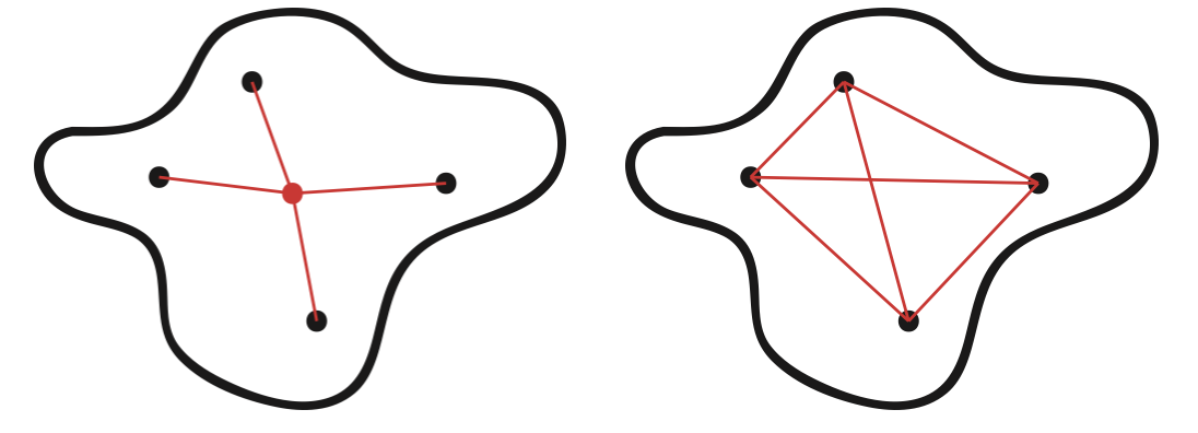
Figure 23.1: Cluster Cohesion in Data (left) compared to Graph-Based Cluster Cohesion (right)
Depending on the proximity or similarity function used, the two quantities in Figure 23.1 may or may not be the same. Often times for graphs and networks, there is no simple way to define a centroid or representative point for a cluster. The particular representation for a cohesion metric will always be dependent on a choice of distance or similarity function. Thus, for graphs we merely define the general concept of cohesion as follows:
Definition 23.1 (General Cluster Cohesion in Graphs) For a graph \(G(V,E)\) with edge weights \(w_{ij}\), and a partition of the vertices into \(k\) disjoint sets \(C=\{C_1,C_2,\dots, C_k\}\), the cohesion of cluster \(C_p\) is \[\mbox{cohesion}(C_p) = \sum_{i,j \in C_p} w_{ij}.\]
Given this definition, it should be clear that if \(w_{ij}\) is a measure of similarity between vertices \(i\) and \(j\) then higher values of cohesion are desired, whereas if \(w_{ij}\) measures distance or dissimilarity then lower values of cohesion are desired.
For data clustering problems, cluster cohesion is similarly defined, only now the similarities or proximities are measured between each point in the cluster and the cluster’s representative point.
Definition 23.2 (General Cluster Cohesion for Data) Let \(\X=[\x_1,\x_2,\dots, \x_n]\) be an \(m\times n\) matrix of column data, and let \(C=\{C_1,C_2,\dots,C_k\}\) be a set of disjoint clusters partitioning the data with corresponding representative points \(\{\cc_1,\cc_2,\dots,\cc_k\}\). Then the cohesion of cluster \(C_p\) is \[\mbox{cohesion}(C_p) = \sum_{\x_i \in C_p} d(\x_i,\cc_p)\] Where \(d\) is any distance or similarity function.
Again, the given definitions are not associated with any particular distance or similarity function and thus define a broad classes of metrics for measuring cluster cohesion.
23.1.0.1 Separation
The goal in clustering is not only to form groups of points which are similar or proximal, but also to assure some level of separation or dissimilarity between these groups. Thus, in addition to measuring cluster cohesion, it is also wise to consider cluster separation. Again this concept is a little different for graphs, where the separation is measured pairwise between points in different clusters, than it is for data, where separation is generally measured between the representative points of different clusters. This difference is presented with the following 2 definitions.
Definition 23.3 (General Cluster Separation for Graphs) For a graph \(G(V,E)\) with edge weights \(w_{ij}\), and a partition of the vertices into \(k\) disjoint sets \(C=\{C_1,C_2,\dots, C_k\}\). The separation between clusters \(C_p\) and \(C_q\) is \[\mbox{separation}(C_p,C_q) = \sum_{\substack{i \in C_p \\ j \in C_q}} w_{i,j}.\]
Definition 23.4 (General Cluster Separation for Data) Let \(\X=[\x_1,\x_2,\dots, \x_n]\) be an \(m\times n\) matrix of column data, and let \(C=\{C_1,C_2,\dots,C_k\}\) be a set of disjoint clusters in the data with corresponding representative points \(\{\cc_1,\cc_2,\dots,\cc_k\}\). Then the separation between clusters \(C_p\) and \(C_q\) is \[\mbox{separation}(C_p,C_q) = d(\cc_p,\cc_q)\] where \(d\) is any distance or similarity function.
23.1.0.2 Averaging Measures of Cohesion and Separation for a Set of Clusters
Definitions 23.1, 23.2, 23.3 and 23.4 provide simple, well-defined metrics (given a proximity or similarity measure) for individual clusters \(C_p\) or pairs of clusters \((C_p,C_q)\) that can be combined into overall measures for a clustering \(C = \{C_1,C_2,\dots,C_k\}\) by some weighted average [54]. The weights for such an average vary according to applications and user-preference, but they typically reflect the size of the clusters in some way. At the end of this chapter, in Table 23.2, we provide a few examples of these overall metrics.
23.1.1 Common Measures of Cohesion and Separation
As stated earlier, the previous definitions were considered “general” in that they did not specify particular functions of similarity or distance. Here we discuss some specific measures which have become established as foundations of cluster validation in the literature.
23.1.1.1 Sum of Squared Error (SSE)
The sum of squared error (SSE) metric incorporates the squared euclidean distances from each point in a given cluster to the centroid of the cluster, defined as \[\mean_j = \frac{1}{n_j} \sum_{\x_i \in C_j} \x_i.\] This is equivalent to measuring the average pairwise distance between points in a cluster, as one would do in a graph having Euclidean distance as a measure of proximity. The SSE of a single cluster is then
\[\begin{eqnarray*} \text{SSE}(C_j)&=&\sum_{\x_i \in C_j} \| \x_i - \mean_j \|_2^2 \\ &=&\frac{1}{2n_j}\sum_{\x_i,\x_l \in C_j} \|\x_i - \x_l\|_2^2 \label{SSE} \end{eqnarray*}\] where \(n_j = |C_j|\) . The SSE of an entire clustering \(C\) is simply the sum of the SSE for each cluster \(C_j \in C\) \[\mbox{SSE}(C)=\sum_{j=1}^k \sum_{\x_i \in C_j} \|\x_i - \mean_j\|_2^2.\]
Smaller values of SSE indicate more cohesive or compact clusters. One may recognize Equation (??) as the objective function from Section 21.2.2 because minimizing the SSE is the goal of the Euclidean algorithm. We can use the same idea to measure cluster separation by computing the Between Group Sums of Squares (SSB), which is a weighted average of the squared distances from the cluster centroids \(\{\mean_1, \mean_2,\dots,\mean_k\}\) to the over all centroid of the dataset \(\mean_* = \frac{1}{n} \sum_{i=1}^n \x_i\): \[ \mbox{SSB}(C) =\sum_{j=1}^k n_j\|\mean_j-\mean_*\|_2^2. \]
It is straightforward to show that the total sum of squares (TSS) of the data \[\mbox{TSS}(\X)=\sum_{i=1}^n \|\x_i-\mean_*\|_2^2,\] which is constant, is equal to the sum of the SSE and SSB for every clustering \(C\), i.e. \[\mbox{TSS}(\X)=\mbox{SSE}(C) + \mbox{SSB}(C),\] thus minimizing the SSE (attaining more cohesion) is equivalent to maximizing the SSB (attaining more separation).
Sum of Squared Error is used as a tool in the calculation of the gap statistic, outlined in the next chapter, a popular parameter used to determine the number of clusters in data.
23.1.1.2 Ray and Turi’s Validity Measure
In [15] a measure of cluster validity is chosen as the ratio of intracluster distance to intercluster distance. The authors define these distances as \[M_{intra} = \frac{1}{n}\mbox{SSE}(C) = \frac{1}{n}\sum_{j=1}^k \sum_{\x_i \in C_j} \|\x_i - \mean_j\|^2.\] and \[M_{inter} = \min_{1\leq i \leq j \leq k} \|\mean_i - \mean_j\|^2.\] Clearly a good clustering should have small \(M_{intra}\) and large \(M_{inter}\). Ray and Turi’s validity measure, \[V=\frac{M_{intra}}{M_{inter}}\] is expected to take on smaller values for a better clustering [16].
23.1.1.3 Silhouette Coefficients
Silhouette coefficients are popular indices that combine the concepts of cohesion and separation [67]. These indices are defined for each object or observation \(\x_i,\, i=1,\dots, n\) in the data set using two parameters \(a_i\) and \(b_i\), measuring cohesion and separation respectively. These parameters and the silhouette coefficient for an object \(\x_i\) are computed as follows:- Suppose, for a given clustering \(C=\{C_1,\dots, \C_k\}\) with \(|C_j|=n_j\), that the point \(\x_i\) belongs to cluster \(C_p\)
- Then \(a_i\) is the average distance (or similarity) of point \(\x_i\) from the other points in \(C_p\), \[ a_i = \frac{1}{n_p} \sum_{\x_j \in C_p} d(\x_i,\x_j)\]
- Define the distance (or similarity) between \(\x_i\) and the remaining clusters \(C_q, 1\leq\,q\leq\,k, q\neq p\) to be the average distance (or similarity) between \(\x_i\) and the points in each cluster, \[d(\x_i,C_q) = \frac{1}{n_q} \sum_{\x_j \in C_q} d(\x_i,\x_j).\] Then \(b_i\) is defined to be the minimum of these distances (or maximum for similarity): \[b_i = \min_{q \neq p} d(\x_i,C_q).\]
-
The silhouette coefficient for \(\x_i\) is then \[s_i = \frac{(b_i-a_i)}{\max(a_i,b_i)} \mbox{ (for distance metrics)}\] \[s_i = \frac{(a_i-b_i)}{\max(a_i,b_i)} \mbox{ (for similarity metrics)}\]
The silhouette coefficient takes on values \(-1 \leq s_i \leq 1\), where negative values undesirably indicate that \(\x_i\) is closer (or more similar) on the average to points in another cluster than to points in its own cluster, and values close to \(1\) indicate a good clustering.\
Silhouette coefficients are commonly averaged for all points in a cluster to get an overall sense for the validity of that cluster.
23.2 External Validity Metrics
Many of the results presented in Chapter ?? will use data sets for which the class labels of each object are known. Using this information, one can generally create validity metrics that are easier to understand and compare across clusterings. Such metrics are known as external metrics because of their dependence on the external class labels. We will show that most external metrics can be transformed into relative metrics which compute the similarity between two clusterings.
Using the information from external class labels, one can create a so-called confusion matrix (also called a matching matrix). The confusion matrix is simply a table that shows correspondence between predicted cluster labels (determined by an algorithm) and the actual or “true” cluster labels of the data. A simple example is given in Figure 23.2, where the actual class labels (science',math’, and `french’) are shown across the columns of the matrix and the clusters determined by an algorithm (\(C_1, C_2,\) and \(C_3\)) are shown along the rows. The \((i,j)^{th}\) entry in the confusion matrix is then the number of objects from the dataset that had class label \(j\) and were assigned to cluster \(i\).
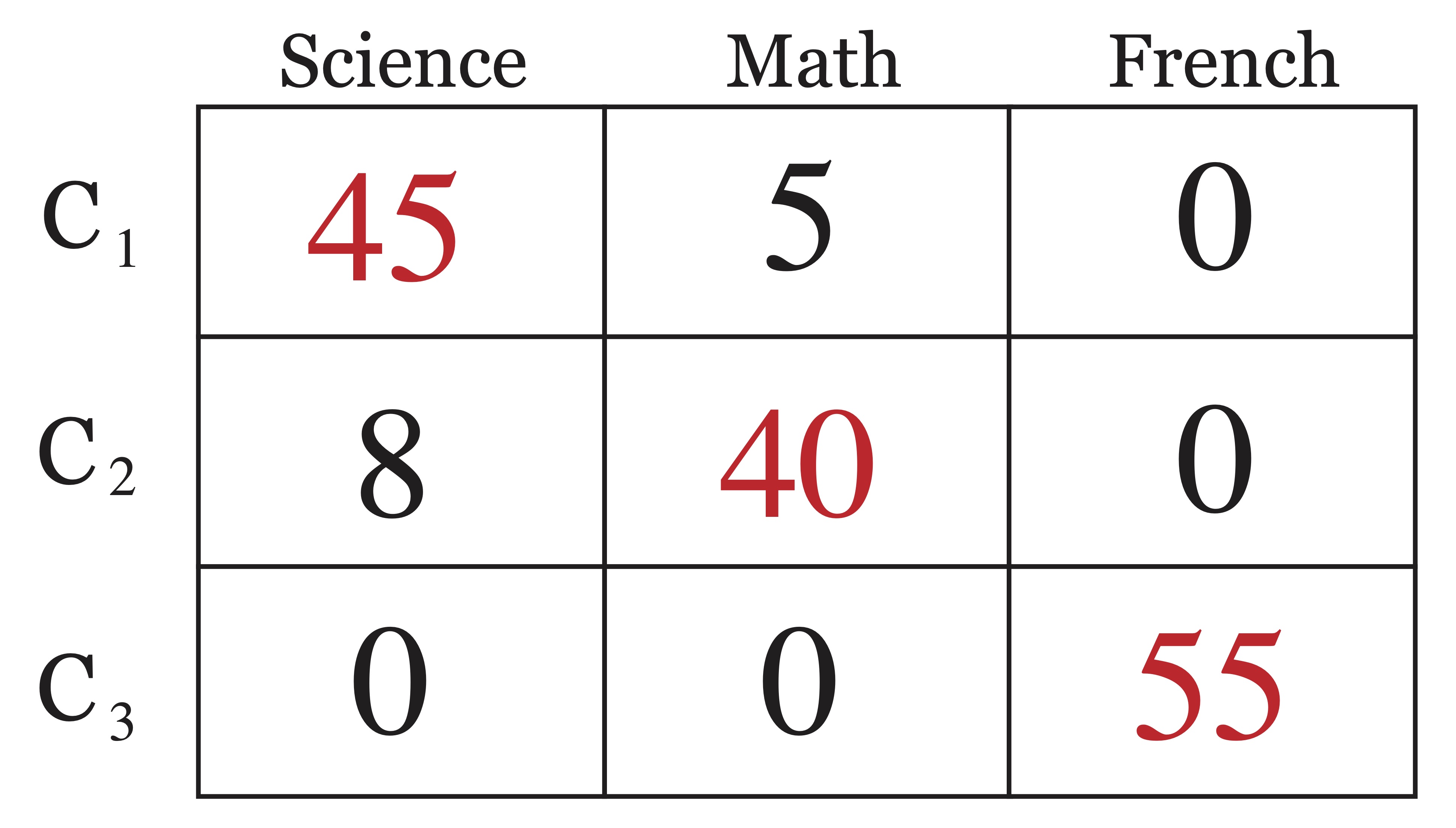
Figure 23.2: Example of a Confusion Matrix
For this simple example, one may assume that cluster 1 (\(C_1\)) corresponds to the class Science', cluster 2 corresponds to the classMath’, and likewise that cluster 3 represents the class `French’, even though the clustering algorithm did not split these classes apart perfectly. Most external metrics will rely on the values in the confusion matrix.
23.2.1 Accuracy
Accuracy is a measure between 0 and 1 that simply measures the proportion of objects that were labelled correctly by an algorithm. This is not always a straightforward task, given that the labels assigned by a clustering algorithm are done so arbitrarily in that it does not matter if one refers to the same group of points as “cluster 1” or “cluster 2.” In the confusion matrix in Figure 23.2, it is easy to identify which cluster labels corresponds to which class. In this case it is easy to see that out of a total of 153 objects, only 13 were classified incorrectly, leading to an accuracy of 140/153 \(\approx\) 91.5%. However with a more confusing confusion matrix, like that shown in Figure 23.3, the answer is not quite as clear and thus it is left to determine exactly how to match predicted cluster labels with assigned class labels in an appropriate way.
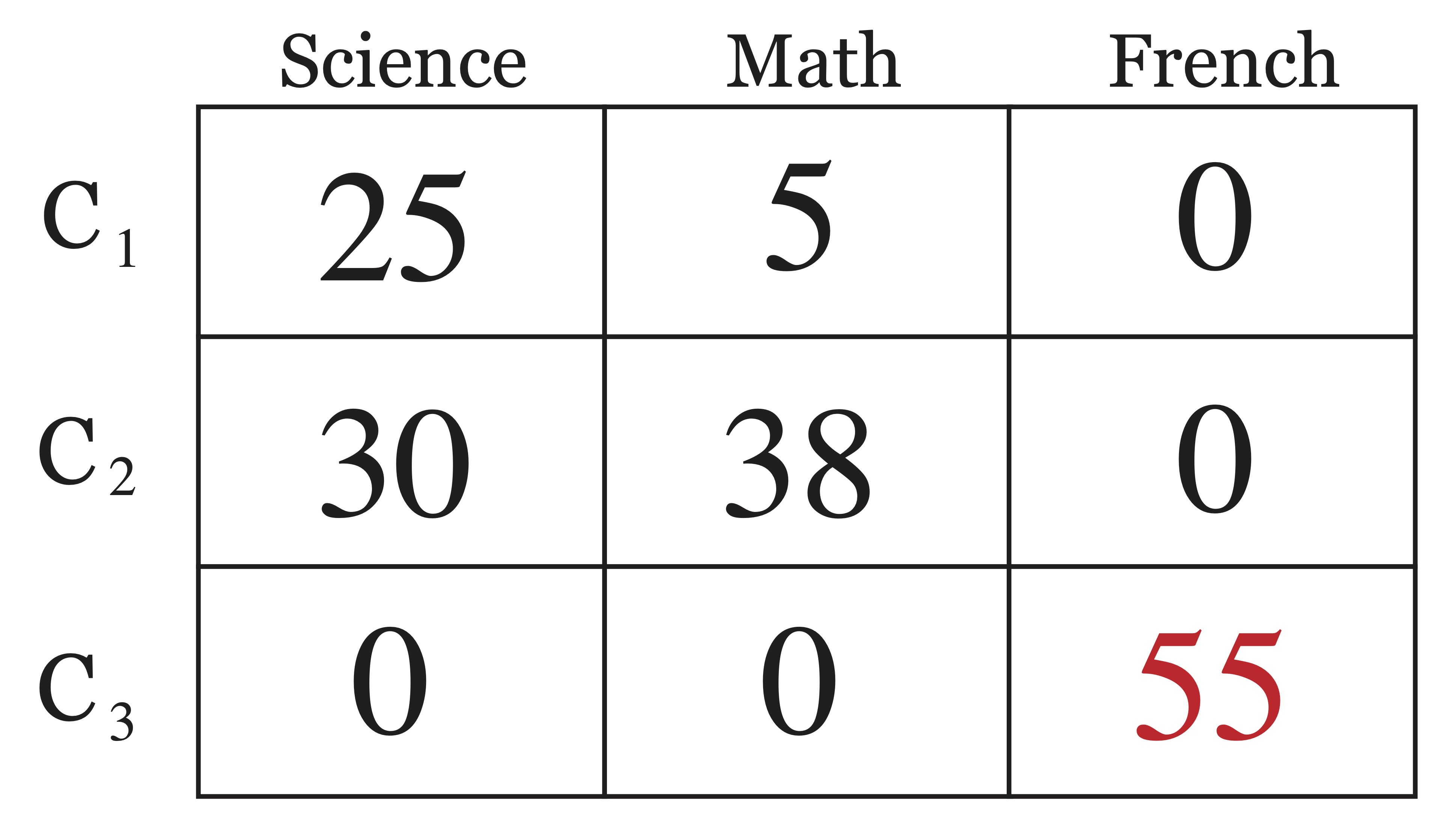
Figure 23.3: A More Confusing Confusion Matrix
This turns out to be a well studied matching problem from graph theory, known as a maximum matching for a bipartite graph. If we transform our confusion matrix from Figure 23.3 into an undirected bipartite graph with edge weights corresponding to edges in the confusion matrix, the result would be the graph in Figure ??. The task is then to find a set of 3 edges, each beginning at distinct vertices on the left and ending at distinct vertices on the right such that the sum of the edge weights is maximal. The solution to this problem is shown in Figure 23.4 and it is clear that the matching of predicted labels to actual labels did not actually change from the simpler version of this confusion matrix in Figure 23.2, it just became less obvious because of the errors made by the algorithm.
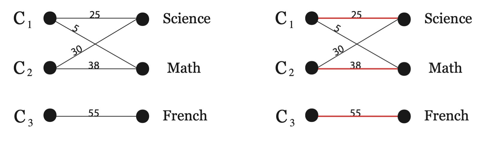
Figure 23.4: Bipartite Graph of Confusion Matrix (left) and Matching Predicted Class Labels to Actual Class Labels (right)
Once the predicted class labels are matched to the actual labels, the accuracy of a clustering is straightforward to compute by \[\mbox{Accuracy}(C)=\frac{\mbox{# of objects labelled correctly}}{n}.\] The accuracy of the second clustering given in Figure 23.3 is 118/153 \(\approx\) 77%, which is sharply lower than the 91.5% achieved by the clustering in Figure 23.2. The nice thing about accuracy as a metric is it provides a contextual interpretation and thus allows us to quantify an answer to the question “how much better is this clustering?” This is not necessarily true of other external metrics, as you will see in the next sections.
The aspect of this metric that requires some computation is the determination of the maximum matching as shown in Figure @ref(fig:bipartitematching}. Fortunately, this problem is one that was solved by graph theorist H.W. Kuhn in 1955 [62]. Kuhn’s algorithm was adapted by James Munkres in 1957 and the resulting method was dubbed the Kuhn-Munkres Algorithm, or sometimes the Hungarian Algorithm in honor of the mathematicians who pioneered the work upon which Kuhn’s method was based [53]. This algorithm is fast and computationally inexpensive. The details of the process are not pertinent to the present discussion, but can be found in any handbook of graph theory algorithms.
23.2.1.1 Comparing Two Clusterings: Agreement
The accuracy metric, along with other external metrics, can be used to compute the similarity between two different cluster solutions. Since, in practice, class labels are not available for the data, the user may run two different clustering algorithms (or even the same algorithm with different representations of the data as input or different initializations) and get two different clusterings as a result. The natural question is then “how similar are these two clusterings?” Treating one clustering as class labels and computing the accuracy of the second compared to the first will provide the percentage of data points for which the two clusterings agree on cluster assignment. Thus, when comparing two clusterings, the accuracy metric becomes a measure of agreement between the two clusterings. As such, value of 90% agreement indicates that 90% of the data points were clustered the same way in both clusterings.
23.2.2 Entropy
The notion of entropy is associated with randomness. As a clustering metric, entropy measures the degree to which the predicted clusters consist of objects belonging to a single class, as opposed to many classes. Suppose a cluster (as predicted by an algorithm) contains objects belonging to multiple classes (as given by the class labels). Define the quantities
- $n_i = $ number of objects in cluster \(C_i\)
- $n_{ij} = $ number of objects in cluster \(C_i\) having class label \(j\)
- $p_{ij} = = $ probability that a member of cluster \(C_i\) belongs to class \(j\)
Then the entropy of each cluster \(C_i\) is \[\mbox{entropy}(C_i) = -\sum_{j=1}^L p_{ij} \log_2 p_{ij}\] where \(L\) is the number of classes, and the total entropy for a set of clusters, \(C\), is the sum of the entropies for each cluster weighted by the proportion of points in that cluster: \[\mbox{entropy}(C)=\sum_{i=1}^k \frac{n_i}{n} \mbox{entropy}(C_i).\]
Smaller values of entropy indicate a less random distribution of class labels within clusters [67]. One benefit of using entropy rather than accuracy is that it can be calculated for any number of clusters \(k\), whereas accuracy is restricted to the case where \(k=L\).
Sample Calculations for Entropy
Comparing the two clusterings represented by the confusion matrices in Figures 23.2 and 23.3, we’d see that for the first example,
\[\begin{eqnarray*} p_{11}=\frac{45}{50} & p_{12}=\frac{5}{50} & p_{13}=0 \\ p_{21}=\frac{8}{48} & p_{22}=\frac{40}{48} & p_{23}=0 \\ p_{31}=0 & p_{32}=0 & p_{33}=1 \end{eqnarray*}\]
so that \[\begin{eqnarray*} \mbox{entropy}(C_1) &=& - ( \frac{45}{50} \log_2 \frac{45}{50} + \frac{5}{50} \log_2 \frac{5}{50}) = 0.469\\ \mbox{entropy}(C_2) &=& - (\frac{8}{48} \log_2 \frac{8}{48} + \frac{40}{48} \log_2 \frac{40}{48}) = 0.65\\ \mbox{entropy}(C_3) &=& - (\log_2 1) = 0 \end{eqnarray*}\] and thus the total entropy of the first clustering is \[\mbox{entropy}(C) = \frac{50}{153} (0.469) + \frac{48}{153}(0.65) = \framebox{0.357}.\]
And for the second example, we have \[\begin{eqnarray*} p_{11}=\frac{25}{30} & p_{12}=\frac{5}{30} & p_{13}=0 \\ p_{21}=\frac{30}{68} & p_{22}=\frac{38}{68} & p_{23}=0 \\ p_{31}=0 & p_{32}=0 & p_{33}=1 \end{eqnarray*}\] yielding \[\begin{eqnarray*} \mbox{entropy}(C_1) &=& - ( \frac{25}{30} \log_2 \frac{25}{30} + \frac{5}{30} \log_2 \frac{5}{30} ) = 0.65 \\ \mbox{entropy}(C_2) &=& - (\frac{30}{68} \log_2 \frac{30}{68} + \frac{38}{68} \log_2 \frac{38}{68}) = 0.99 \\ \mbox{entropy}(C_3) &=& - (\log_2 1) = 0 \end{eqnarray*}\] and finally the total entropy of the second clustering is \[\mbox{entropy}(C) = \frac{30}{153} (0.469) + \frac{68}{153}(0.65) = \framebox{0.568}\]
revealing a higher-overall entropy and thus a worse partition of the data compared to the first clustering.
23.2.3 Purity
Purity is a simple measure of the extent to which a predicted cluster contains objects of a single class [67]. Using the quantities defined in the previous section, the purity of a cluster is defined as \[\mbox{purity}(C_i) = \max_j p_{ij}\] and the purity of a clustering \(C\) is the weighted average \[\mbox{purity}(C) = \sum_{i=1}^k \frac{n_i}{n} \mbox{purity}(C_i).\] The purity metric takes on positive values less than 1, where values of 1 reflect the desirable situation where each cluster only contains objects from a single class. Like entropy, purity can be computed for any number of clusters, \(k\). Purity and accuracy are often confused and used interchangeably but they are not the same. Purity takes no matching of class labels to cluster labels into account, and thus it is possible for the purity of two clusters to count the proportion of objects having the same class label. For example, suppose we had only two class labels given, A and B, for a set of 10 objects and set our clustering algorithm to seek 2 clusters in the data and the following confusion matrix resulted:
Then the purity of each cluster would be \(\frac{3}{5}\) referring in both cases to the proportion of objects having class label A. High values of purity are easy to achieve when the number of clusters is large. For example, by assigning each object to its own cluster we’d achieve perfect purity. One metric that accounts for such a tradeoff is Normalized Mutual Information, presented next.
Sample Purity Calculations
Again, we’ll compare the two clusterings represented by the confusion matrices in Figures 23.2 and 23.3. For the first clustering,
\[\begin{eqnarray*}
\mbox{purity}(C_1) &=& \max(\frac{45}{50} ,\frac{5}{50} ,0) = \frac{45}{50}= 0.9 \\
\mbox{purity}(C_2) &=& \max(\frac{8}{48},\frac{40}{48},0) = \frac{40}{48} = 0.83 \\
\mbox{purity}(C_2) &=& \max(0,0,1) = 1
\end{eqnarray*}\]
so the overall purity is
\[\mbox{purity}(C) = \frac{50}{153} (0.9) + \frac{48}{153}(0.83) + \frac{55}{153}(1) = \framebox{0.914}.\]
Similarly for the second clustering we have, \[\begin{eqnarray*} \mbox{purity}(C_1) &=& \max(\frac{25}{30},\frac{5}{30},0) = \frac{25}{30}) = 0.83 \\ \mbox{purity}(C_2) &=& \max(\frac{30}{68},\frac{38}{68} ,0) = \frac{38}{68}) = 0.56 \\ \mbox{purity}(C_2) &=& \max(0,0,1) = 1 \end{eqnarray*}\]
And thus the overall purity is \[\mbox{purity}(C) = \frac{30}{153} (0.83) + \frac{68}{153}(0.56) + \frac{55}{153}(1) = \framebox{0.771}.\]
23.2.4 Mutual Information (MI) and
Normalized Mutual Information (NMI)
Mutual Information (MI) is a measure that has been used in various data applications [67]. The objective of this metric is to measure the amount information about the class labels revealed by a clustering. Adopting the previous notation,
- $n_i = $ number of objects in cluster \(C_i\)
- $n_{ij} = $ number of objects in cluster \(C_i\) having class label \(j\)
- $p_{ij} = n_{ij}/n_i = $ probability that a member of cluster \(C_i\) belongs to class \(j\)
also let
- \(l_j =\) the number of objects having class label \(j\)
- \(L =\) the number of classes
- \(\mathcal{L} =\{\mathcal{L}_1,\dots,\mathcal{L}_L\}\) the “proper” clustering according to class labels
- \(n=\) the number of objects in the data
- \(k=\) the number of clusters in the clustering.
The Mutual Information of a clustering \(C\) is then \[\mbox{MI}(C)=\sum_{i=1}^k \sum_{j=1}^L p_{ij} \log \frac{n n_{ij}}{n_i l_j}\] and the Normalized Mutual Information of \(C\) is \[\mbox{NMI}(C) = \frac{\mbox{MI}(C)}{[\mbox{entropy}(C) + \mbox{entropy}(\mathcal{L})]/2}\] Clearly, when \(\mathcal{L}\) corresponds the class labels we have \(\mbox{entropy}(\mathcal{L})=0\) but if user’s objective is instead to compare two different clusterings, this piece of the equation is necessary. Thus, using the same treatment used for agreement between two clusterings, one can compute the mutual information between two clusterings.
23.2.5 Other External Measures of Validity
There are a number of other measures that can either be used to validate a clustering in the presence of class labels or to compare the similarity between two clusterings \(C=\{C_1,C_2,\dots,C_k\}\) and \(\hat{C}=\{\hat{C}_1,\hat{C}_2,\dots,\hat{C_k}\}\). In our presentation we will consider the second clustering to correspond to the class labels, but in the same way that the accuracy metric can be used to compute agreement, these measures are often used to compare different clusterings. To begin we define the following parameters [16]:- \(a\) is the number of pairs of data points which are in the same cluster in \(C\) and have the same class labels (i.e. are in the same cluster in \(\hat{C}\)).
- \(b\) is the number of pairs of data points which are in the same cluster in \(C\) and have different class labels.
- \(c\) is the number of pairs of data points which are in different clusters in \(C\) and have the same class labels.
- \(d\) is the number of pairs of data points which are in different clusters in \(C\) and have different class labels.
These four parameters add up to the total number of pairs of points in the data set, \(N\), \[a+b+c+d = N = \frac{n(n-1)}{2}.\]
From these values we can compute a number of different similarity coefficients, a few of which are provided in Table 23.1 [16].
| Name | Formula |
| Jaccard Coefficient | \(\displaystyle J = \frac{a}{a+b+c}\) |
| Rand Statistic | \(\displaystyle R = \frac{a+b}{N}\) |
| Folkes and Mallows Index | \(\displaystyle \sqrt{\frac{a}{a+b} \frac{a}{a+c}}\) |
| Odds Ratio | \(\displaystyle \frac{ad}{bc}\) |
23.2.5.1 Hubert’s \(\Gamma\) Statistic
Another measure popular in the clustering literature is Hubert’s \(\Gamma\) statistic, which aims to measure the correlation between two clusterings, or between one clustering and the class label solution [16], [67]. Here we define an \(n\times n\) adjacency matrix for a clustering \(C\), denoted \(\bo{Y}\) such that
\[\begin{equation} \label{clusteradjacency} \bo{Y}_{ij} = \begin{cases} 1 & \text{object } i \text{ and object } j \text{ are in the same cluster in } C \\ 0 & \text{otherwise} \end{cases} \end{equation}\]
Similarly, let \(\bo{H}\) be an adjacency matrix pertaining to the class label partition (or a different clustering) as follows: \[\begin{equation} \bo{H}_{ij} = \begin{cases} 1 & \mbox{object } i \mbox{ and object } j \mbox{ have the same class label } \\ 0 & \mbox{otherwise} \end{cases} \end{equation}\]
Then Hubert’s \(\Gamma\) statistic, defined as \[\Gamma=\frac{1}{N} \sum_{i=1}^{n-1} \sum_{i+1}^n \bo{Y}_{ij} H_{ij},\] is a way of measuring the correlation between the clustering and the class label partition [16].
23.2.6 Summary Table
| Name | Overall Measure | Cluster Weight | Type | Overall Cohesion (Graphs) | ${p=1}^k p {i,j C_p} w{ij} $ | \(\displaystyle \alpha_p= \frac{1}{n_i}\) | Graph Cohesion | \(\mathcal{G}_{CS}\) (Graph C-S Measure) | \(\displaystyle\sum_{p=1}^k \alpha_p \sum_{\substack{q=1 \\ q\neq p}}^k \sum_{\substack{i \in C_p \\ j \in C_q}} w_{ij}\) | \(\displaystyle\alpha_p = \frac{1}{\sum_{i,j \in C_p} w_{ij}}\) | Graph Cohesion & Separation | Sum Squared Error (SSE) (Data) | \(\displaystyle \sum_{p=1}^k \alpha_p \sum_{\x_i\in C_p} \|\x_i - \mean_p\|^2\) | \(\displaystyle\alpha_p = 1\) | Data Cohesion | Ray and Turi’s \(M_{intra}\) | \(\displaystyle \sum_{p=1}^k \alpha_p \sum_{\x_i\in C_p} \|\x_i - \mean_p\|^2\) | \(\displaystyle\alpha_p = \frac{1}{n}\) | Data Cohesion | Ray and Turi’s \(M_{inter}\) | $_{1i j k} |_i - _j|^2 $ | N/A | Data Separation | Ray and Turi’s Validity Measure | \(\displaystyle\frac{M_{intra}}{M_{inter}}\) | N/A | Data Cohesion & Separation |