Chapter 18 Dimension Reduction for Visualization
18.1 Multidimensional Scaling
Multidimensional scaling is a technique which aims to represent higher-dimensional data in a lower-dimensional space while keeping the pairwise distances between points as close to their original distances as possible. It takes as input a distance matrix, \(\D\) where \(\D_{ij}\) is some measure of distance between observation \(i\) and observation \(j\) (most often Euclidean distance). The original observations may involve many variables and thus exist in a high-dimensional space. The output of MDS is a set of coordinates, usually in 2-dimensions for the purposes of visualization, such that the Euclidean distance between observation \(i\) and observation \(j\) in the new lower-dimensional representation is an approximation to \(\D_{ij}\).
One of the outputs in R will be a measure that is akin to the “percentage of variation explained” by PCs. The difference is that the matrix we are representing is not a covariance matrix, so this ratio is not a percentage of variation. It can, however, be used to judge how much information is retained by the lower dimensional representation. This is output in the GOF vector (presumably standing for Goodness of Fit). The first entry in GOF gives the ratio of the sum of the \(k\) largest eigenvalues to the sum of the absolute values of all the eigenvalues, and the second entry in GOF gives the ratio of the sum of the \(k\) largest eigenvalues to the sum of only the positive eigenvalues.
\[GOF[1] = \frac{\sum_{i=1}^k \lambda_i}{\sum_{i=1}^n |\lambda_i|}\] and \[GOF[2] = \frac{\sum_{i=1}^k \lambda_i}{\sum_{i=1}^n \max(\lambda_i,0)}\]
18.1.1 MDS of Iris Data
Let’s take a dataset we’ve already worked with, like the iris dataset, and see how this is done. Recall that the iris data contains measurements of 150 flowers (50 each from 3 different species) on 4 variables: Sepal.Length, Sepal.Width, Petal.Length, and Petal.Width. To examine a 2-dimensional representation of this data via Multidimensional Scaling, we simply compute a distance matrix and run the MDS procedure:
D = dist(iris[,1:4])
fit = cmdscale(D, eig=TRUE, k=2) # k is the number of dimensions desired
fit$eig[1:12] # view first dozen eigenvalues
## [1] 6.3001e+02 3.6158e+01 1.1653e+01 3.5514e+00 3.4866e-13 3.1863e-13
## [7] 2.0112e-13 1.3770e-13 7.7470e-14 3.2881e-14 3.0740e-14 2.1786e-14fit$GOF # view the Goodness of Fit measures## [1] 0.97769 0.97769# plot the solution, colored by iris species:
x = fit$points[,1]
y = fit$points[,2]
# The pch= option controls the symbol output. 16=filled circles.
plot(x,y,col=c("red","green3","blue")[iris$Species], pch=16,
xlab='Coordinate 1', ylab='Coordinate 2')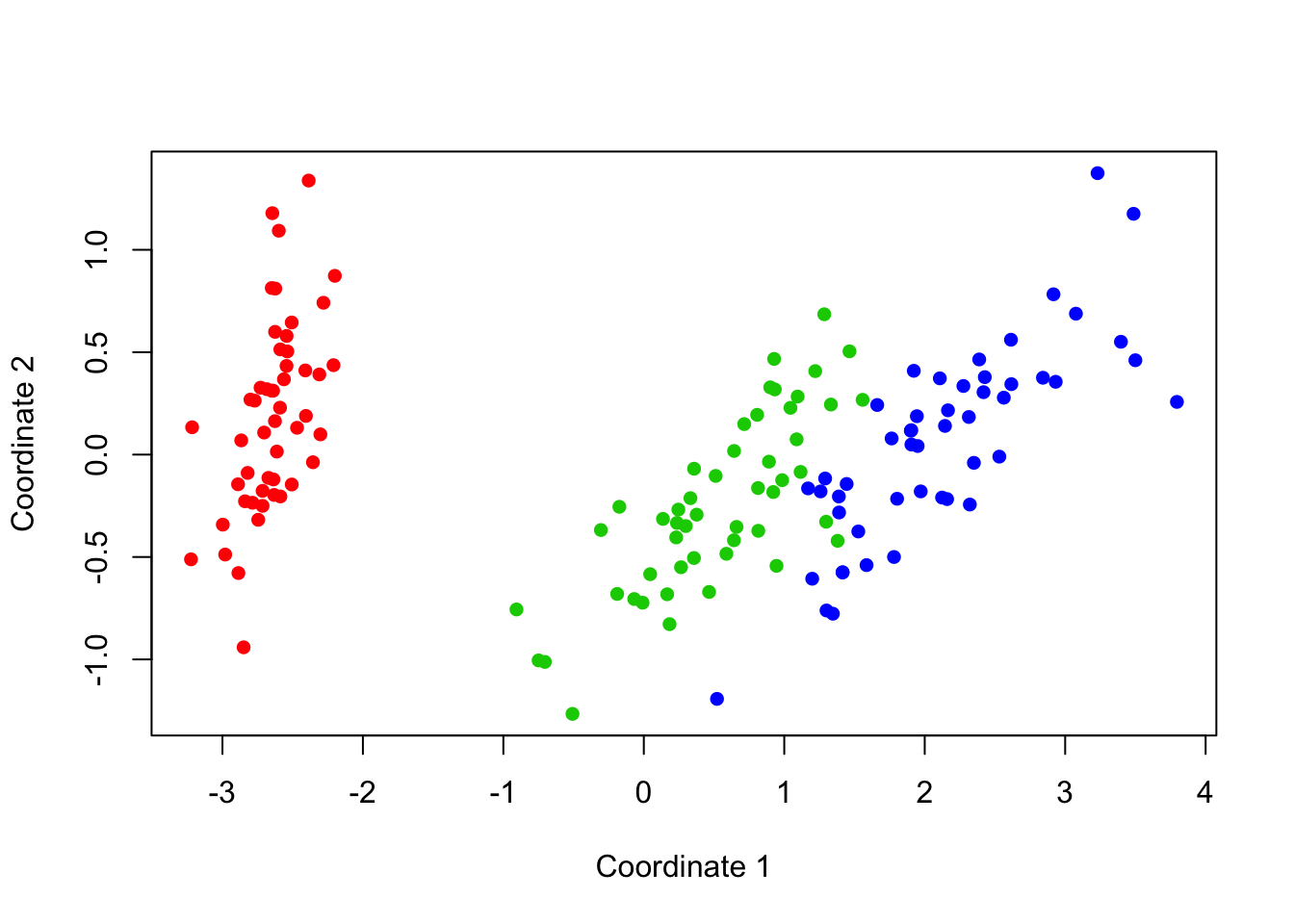
Figure 18.1: Multidimensional Scaling of the Iris Data
We can tell from the eigenvalues alone that two dimensions should be relatively sufficient to summarize this data. After two large eigenvalues, the remainder drop off and become small, signifying a lack of further information. Indeed, the Goodness of Fit measurements back up this intuition: values close to 1 indicate a good fit with minimal error.
18.1.2 MDS of Leukemia dataset
Let’s take a look at another example, this time using the Leukemia dataset which has 5000 variables. It is unreasonable to expect that we can get as good of a fit of this data using only two dimensions! There will obviously be much more error. However, we can still get a visualization that should at least show us which observations are close to each other and which are far away.
leuk=read.csv('http://birch.iaa.ncsu.edu/~slrace/Code/leukemia.csv')As you may recall, this data has some variables with 0 variance; those entire columns are constant. To determine which ones, we first remove the last column which is a character vector that identifies the type of leukemia.
type = leuk[ , 5001]
leuk = leuk[,1:5000]
# If desired, could supply names of columns that have 0 variance with
# names(leuk[, sapply(leuk, function(v) var(v, na.rm=TRUE)==0)])
# The na.rm=T would allow us to keep any missing information and still compute
# the variance using the non-missing values. In this instance, it is not necessary
# because we have no missing values.

# We can remove these columns from the data with:
leuk=leuk[,apply(leuk, 2, var, na.rm=TRUE) != 0]

# compute distances matrix
t=dist(leuk)
fit=cmdscale(t,eig=TRUE, k=2)

fit$GOF
## [1] 0.35822 0.35822x = fit$points[,1]
y = fit$points[,2]
#The cex= controls the size of the circles in the plot function.
plot(x,y,col=c("red","green","blue")[factor(type)], cex=3,
xlab='Coordinate 1', ylab='Coordinate 2',
main = 'Multidimensional Scaling of Raw Leukemia Data')
text(x,y,labels=row.names(leuk))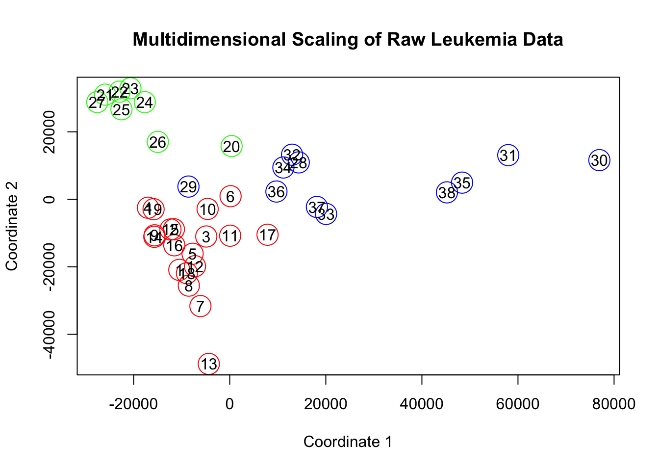
Figure 18.2: Multidimensional Scaling of the Leukemia Data
What if we standardize our data before running the MDS procedure? Will that effect our results? Let’s see how it looks on the standardized version of the leukemia data.
# We can experiment with standardization to see how it
# effects our results:

leuk2=scale(leuk,center=TRUE, scale=TRUE)
t2=dist(leuk2)
fit2=cmdscale(t2,eig=TRUE,k=2)
fit2$GOF
## [1] 0.21287 0.21287x2 = fit2$points[,1]
y2 = fit2$points[,2]
#The cex= controls the size of the circles in the plot function.
plot(x2,y2,col=c("red","green","blue")[factor(type)], cex=3,
xlab='Coordinate 1', ylab='Coordinate 2',
main = 'Multidimensional Scaling of Standardized Leukemia Data')
text(x2,y2,labels=row.names(leuk))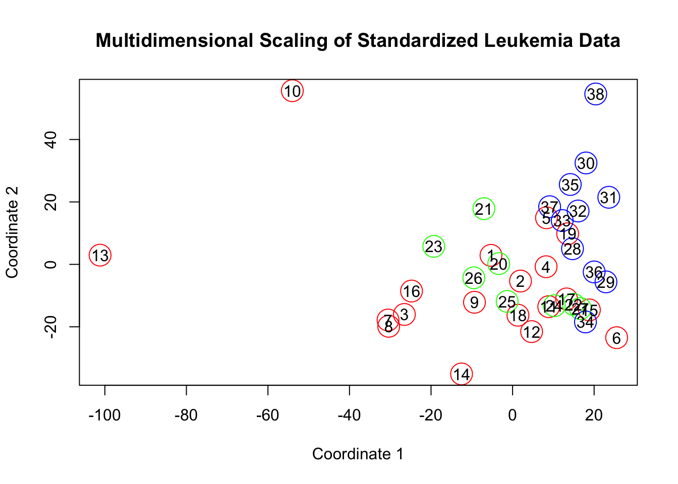
A note on standardization
Clearly, things have changed substantially. We shouldn’t give to much creedence to the decreased Goodness of Fit statistics. I don’t necessarily believe that we are explaining less information just because we scaled our data, the fact that this number has changed should likely be attributed to the fact that we have significantly decreased all of the eigenvalues of the matrix, and not in any predictable or meaningful way. It’s more important to focus on what we are trying to represent and that is differences between samples. Perhaps if there are some genes for which values vary wildly between the different leukemia types, and other genes which don’t show much variation, then we should keep this information in the data. By standardizing the data, we’re making the variation of every gene equal to 1 - which stands to wash out some of the bigger, more discriminating factors in the distance calculations. This consideration is something that will need to be made for each dataset on a case-by-case basis. If our dataset had variables with wide scale variations (like income and number of cars) then standardization is a much more reasonable approach!
There are several things to keep in mind when studying an MDS map.
- The axis are, by themselves, meaningless.
- The orientation of the picture is completely arbitrary.
- All that matters is the relative proximity of the points in the map. Are they close? Are they far apart?