Chapter 14 Applications of Principal Components
Principal components have a number of applications across many areas of statistics. In the next sections, we will explore their usefulness in the context of dimension reduction.
14.1 Dimension reduction
It is quite common for an analyst to have too many variables. There are two different solutions to this problem:
- Feature Selection: Choose a subset of existing variables to be used in a model.
- Feature Extraction: Create a new set of features which are combinations of original variables.
14.1.1 Feature Selection
Let’s think for a minute about feature selection. What are we really doing when we consider a subset of our existing variables? Take the two dimensional data in Example ?? (while two-dimensions rarely necessitate dimension reduction, the geometrical interpretation extends to higher dimensions as usual!). The centered data appears as follows:
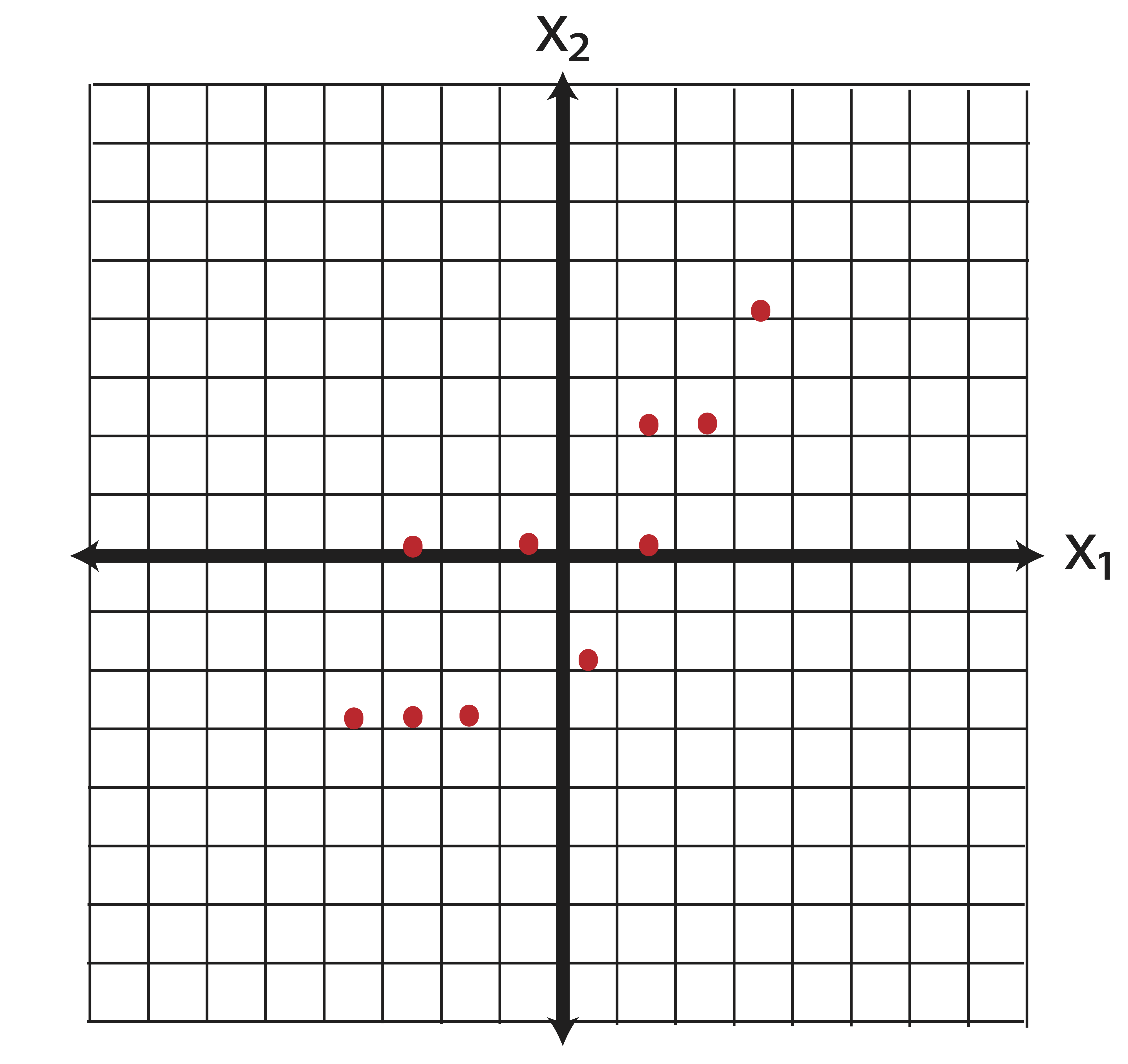
Now say we perform some kind of feature selection (there are a number of ways to do this, chi-square tests for instances) and we determine that the variable \(\x_2\) is more important than \(\x_1\). So we throw out \(\x_2\) and we’ve reduced the dimensions from \(p=2\) to \(k=1\). Geometrically, what does our new data look like? By dropping \(\x_1\) we set all of those horizontal coordinates to zero. In other words, we project the data orthogonally onto the \(\x_2\) axis, as illustrated in Figure 14.1.
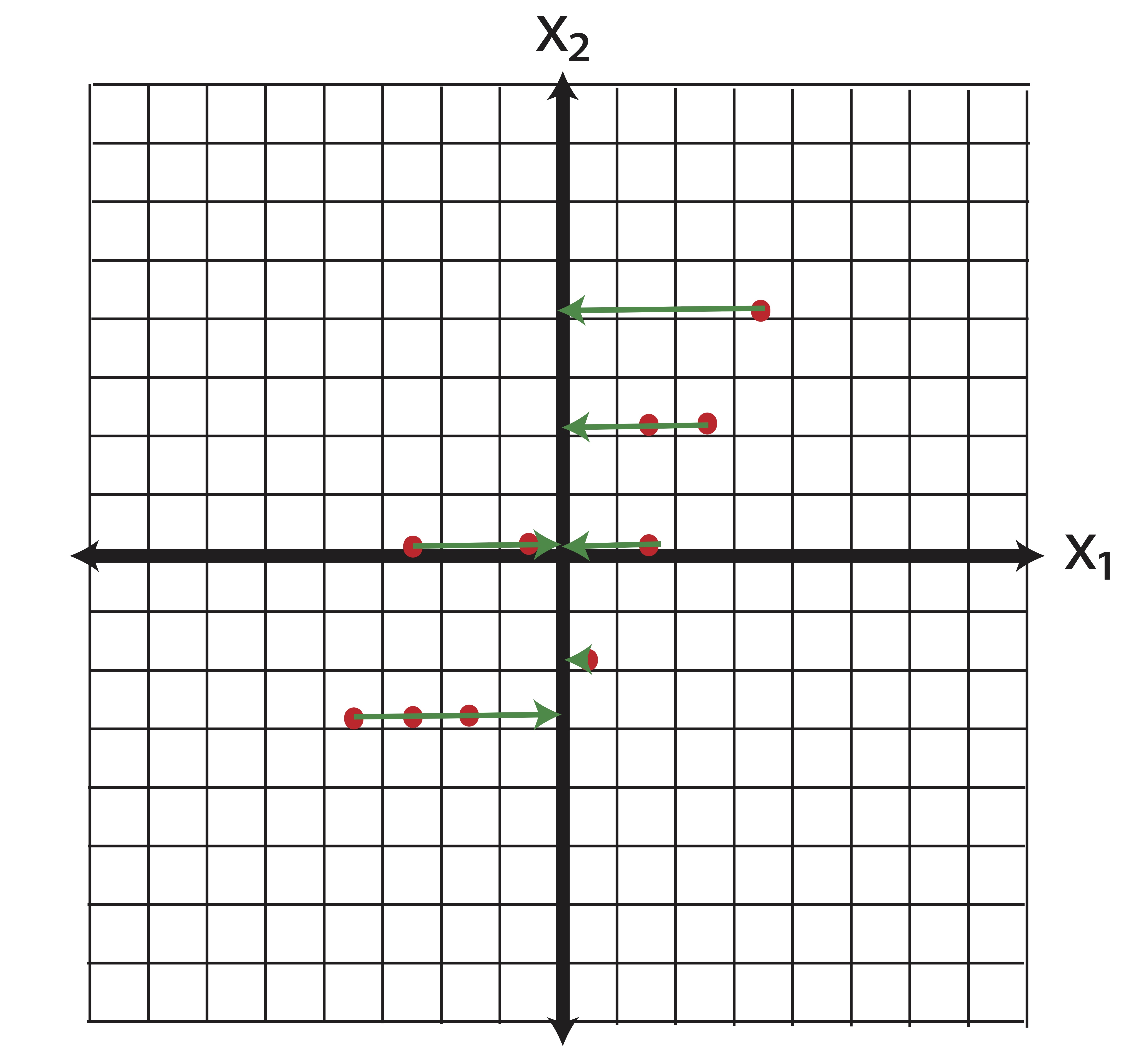
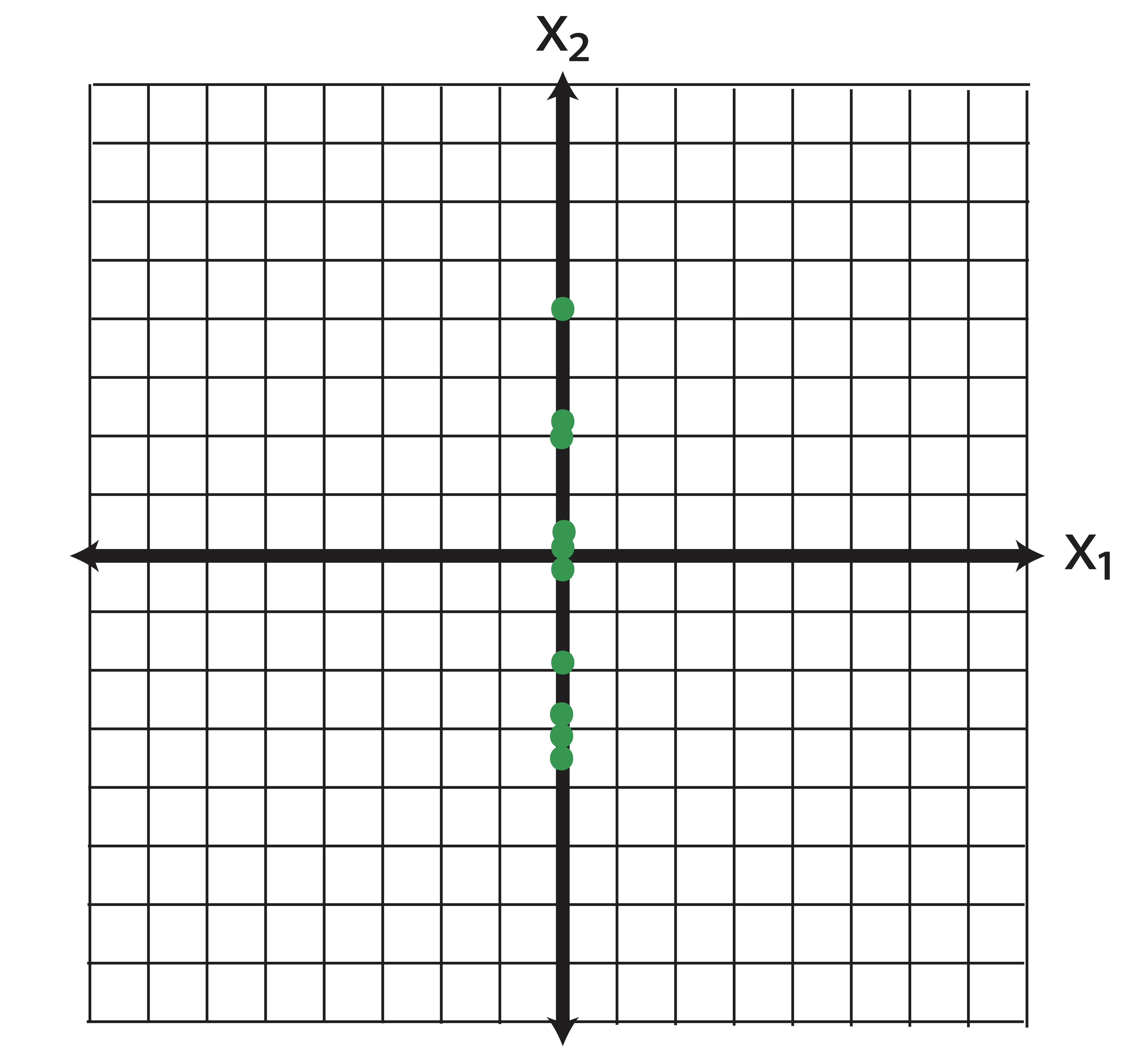
Figure 14.1: Geometrical Interpretation of Feature Selection: When we “drop” the variable \(\x_1\) from our analysis, we are projecting the data onto the span(\(\x_2\))
Now, how much information (variance) did we lose with this projection? The total variance in the original data is \[\|\x_1\|^2+\|\x_2\|^2.\] The variance of our data reduction is \[\|\x_2\|^2.\] Thus, the proportion of the total information (variance) we’ve kept is \[\frac{\|\x_2\|^2}{\|\x_1\|^2+\|\x_2\|^2}=\frac{6.01}{5.6+6.01} = 51.7\%.\] Our reduced dimensional data contains only 51.7% of the variance of the original data. We’ve lost a lot of information!
The fact that feature selection omits variance in our predictor variables does not make it a bad thing! Obviously, getting rid of variables which have no relationship to a target variable (in the case of supervised modeling like prediction and classification) is a good thing. But, in the case of unsupervised learning techniques, where there is no target variable involved, we must be extra careful when it comes to feature selection. In summary,
-
Feature Selection is important. Examples include:
- Removing variables which have little to no impact on a target variable in supervised modeling (forward/backward/stepwise selection).
- Removing variables which have obvious strong correlation with other predictors.
- Removing variables that are not interesting in unsupervised learning (For example, you may not want to use the words “the” and “of” when clustering text).
- Feature Selection is an orthogonal projection of the original data onto the span of the variables you choose to keep.
-
Feature selection should always be done with care and justification.
- In regression, could create problems of endogeneity (errors correlated with predictors - omitted variable bias).
- For unsupervised modelling, could lose important information.
<.ol>
14.1.2 Feature Extraction
PCA is the most common form of feature extraction. The rotation of the space shown in Example ?? represents the creation of new features which are linear combinations of the original features. If we have \(p\) potential variables for a model and want to reduce that number to \(k\), then the first \(k\) principal components combine the individual variables in such a way that is guaranteed to capture as much ``information’’ (variance) as possible. Again, take our two-dimensional data as an example. When we reduce our data down to one-dimension using principal components, we essentially do the same orthogonal projection that we did in Feature Selection, only in this case we conduct that projection in the new basis of principal components. Recall that for this data, our first principal component \(\v_1\) was \[\v_1 = \pm 0.69 \\0.73 \mp.\] Projecting the data onto the first principal component is illustrated in Figure 14.2.
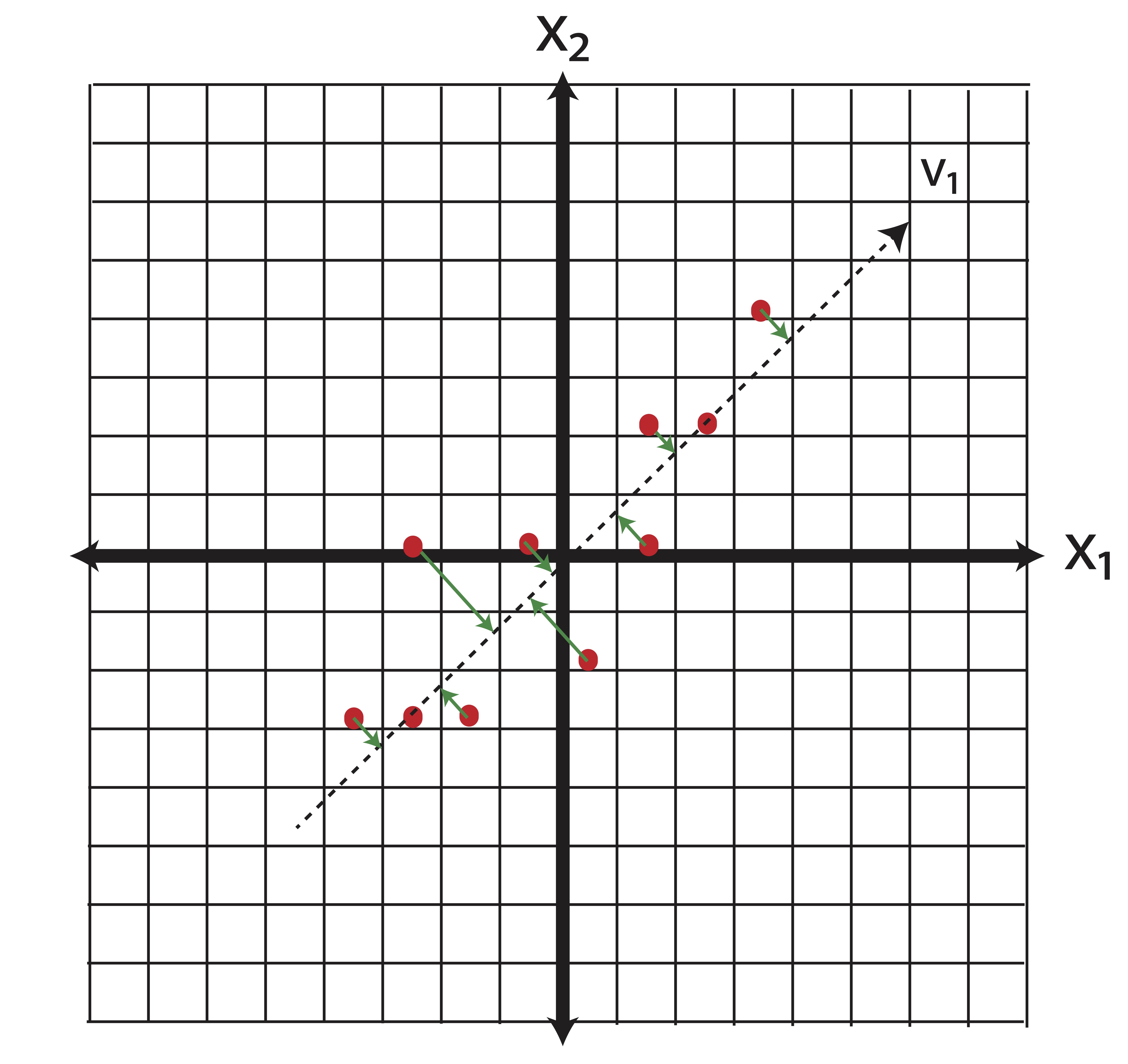
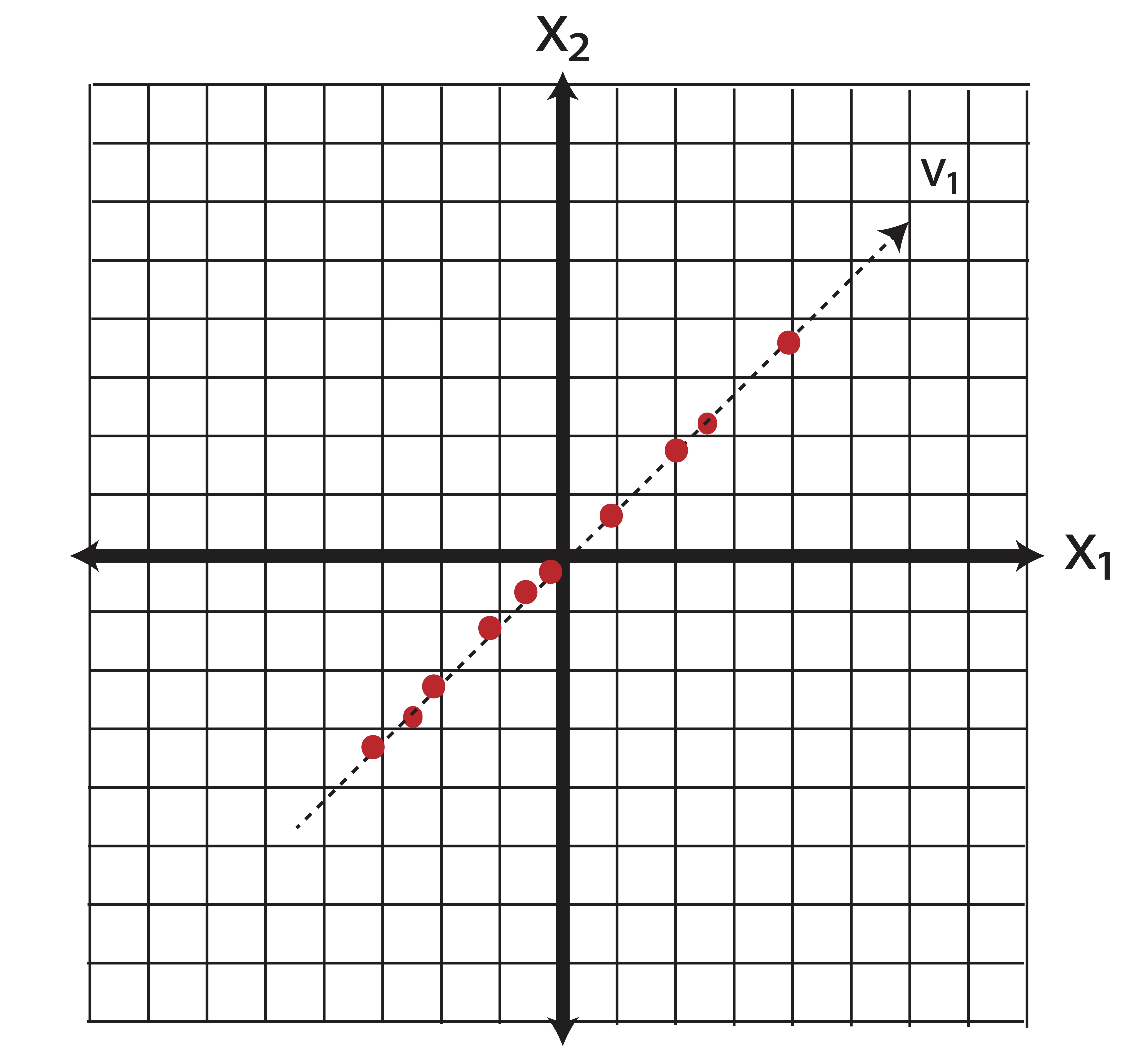
Figure 14.2: Illustration of Feature Extraction via PCA
How much variance do we keep with \(k\) principal components? The proportion of variance explained by each principal component is the ratio of the corresponding eigenvalue to the sum of the eigenvalues (which gives the total amount of variance in the data).
:::{theorem name=‘Proportion of Variance Explained’ #pcpropvar} The proportion of variance explained by the projection of the data onto principal component \(\v_i\) is \[\frac{\lambda_i}{\sum_{j=1}^p \lambda_j}.\] Similarly, the proportion of variance explained by the projection of the data onto the first \(k\) principal components (\(k<j\)) is \[ \frac{\sum_{i=1}^k\lambda_i}{\sum_{j=1}^p \lambda_j}\] :::
In our simple 2 dimensional example we were able to keep \[\frac{\lambda_1}{\lambda_1+\lambda_2}=\frac{10.61}{10.61+1.00} = 91.38\%\] of our variance in one dimension.
14.2 Exploratory Analysis
14.2.1 UK Food Consumption
14.2.1.1 Explore the Data
The data for this example can be read directly from our course webpage. When we first examine the data, we will see that the rows correspond to different types of food/drink and the columns correspond to the 4 countries within the UK. Our first matter of business is transposing this data so that the 4 countries become our observations (i.e. rows).
food=read.csv("http://birch.iaa.ncsu.edu/~slrace/LinearAlgebra2021/Code/ukfood.csv",
header=TRUE,row.names=1)library(reshape2) #melt data matrix into 3 columns
library(ggplot2) #heatmap
head(food)## England Wales Scotland N.Ireland
## Cheese 105 103 103 66
## Carcass meat 245 227 242 267
## Other meat 685 803 750 586
## Fish 147 160 122 93
## Fats and oils 193 235 184 209
## Sugars 156 175 147 139food=as.data.frame(t(food))
head(food)## Cheese Carcass meat Other meat Fish Fats and oils Sugars
## England 105 245 685 147 193 156
## Wales 103 227 803 160 235 175
## Scotland 103 242 750 122 184 147
## N.Ireland 66 267 586 93 209 139
## Fresh potatoes Fresh Veg Other Veg Processed potatoes Processed Veg
## England 720 253 488 198 360
## Wales 874 265 570 203 365
## Scotland 566 171 418 220 337
## N.Ireland 1033 143 355 187 334
## Fresh fruit Cereals Beverages Soft drinks Alcoholic drinks
## England 1102 1472 57 1374 375
## Wales 1137 1582 73 1256 475
## Scotland 957 1462 53 1572 458
## N.Ireland 674 1494 47 1506 135
## Confectionery
## England 54
## Wales 64
## Scotland 62
## N.Ireland 41Next we will visualize the information in this data using a simple heat map. To do this we will standardize and then melt the data using the reshape2 package, and then use a ggplot() heatmap.
food.std = scale(food, center=T, scale = T)
food.melt = melt(food.std, id.vars = row.names(food.std), measure.vars = 1:17)
ggplot(data = food.melt, aes(x=Var1, y=Var2, fill=value)) +
  geom_tile(color = "white")+
  scale_fill_gradient2(low = "blue", high = "red", mid = "white",
                       midpoint = 0, limit = c(-2,2), space = "Lab"
                       ) +  theme_minimal()+
  theme(axis.title.x = element_blank(),axis.title.y = element_blank(),
        axis.text.y = element_text(face = 'bold', size = 12, colour = 'black'),
        axis.text.x = element_text(angle = 45, vjust = 1, face = 'bold',
                                   size = 12, colour = 'black', hjust = 1))+coord_fixed()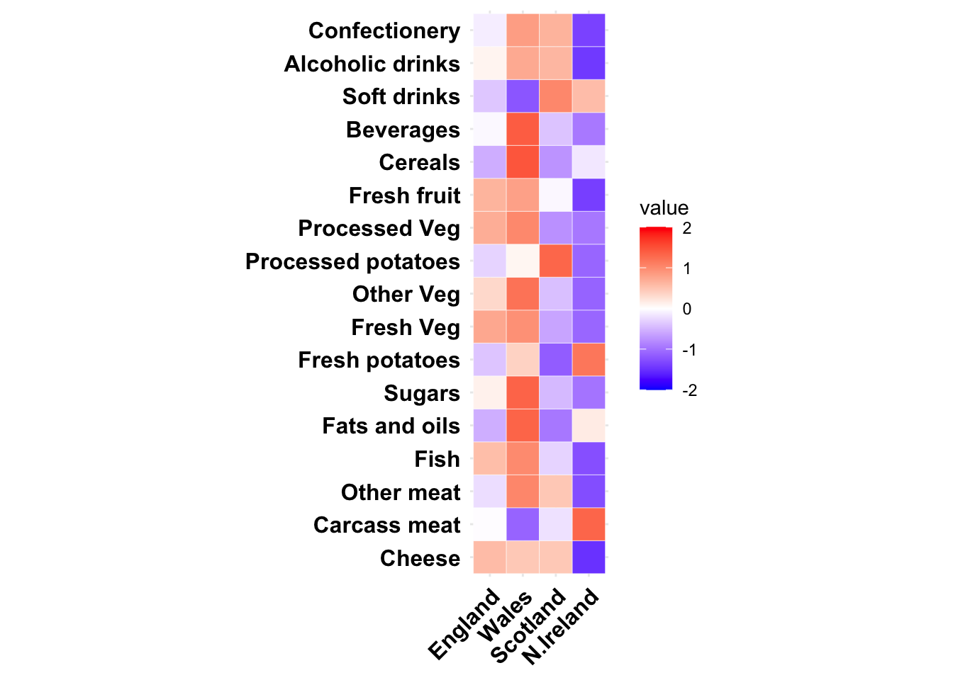
14.2.1.2 prcomp() function for PCA
The prcomp() function is the one I most often recommend for reasonably sized principal component calculations in R. This function returns a list with class “prcomp” containing the following components (from help prcomp):
-
sdev: the standard deviations of the principal components (i.e., the square roots of the eigenvalues of the covariance/correlation matrix, though the calculation is actually done with the singular values of the data matrix). -
rotation: the matrix of variable loadings (i.e., a matrix whose columns contain the eigenvectors). The function princomp returns this in the element loadings. -
x: if retx is true the value of the rotated data (i.e. the scores) (the centred (and scaled if requested) data multiplied by the rotation matrix) is returned. Hence, cov(x) is the diagonal matrix \(diag(sdev^2)\). For the formula method, napredict() is applied to handle the treatment of values omitted by the na.action. -
center,scale: the centering and scaling used, or FALSE.
The option scale = TRUE inside the prcomp() function instructs the program to use orrelation PCA. The default is covariance PCA.
pca=prcomp(food, scale = T) This first plot just looks at magnitudes of eigenvalues - it is essentially the screeplot in barchart form.
summary(pca)## Importance of components:
## PC1 PC2 PC3 PC4
## Standard deviation 3.4082 2.0562 1.07524 6.344e-16
## Proportion of Variance 0.6833 0.2487 0.06801 0.000e+00
## Cumulative Proportion 0.6833 0.9320 1.00000 1.000e+00plot(pca, main = "Bar-style Screeplot")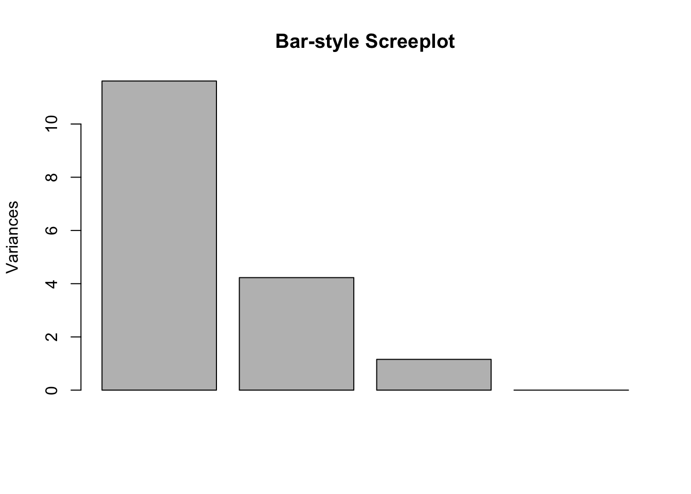
The next plot views our four datapoints (locations) projected onto the 2-dimensional subspace (from 17 dimensions) that captures as much information (i.e. variance) as possible.
plot(pca$x,
     xlab = "Principal Component 1",
     ylab = "Principal Component 2",
     main = 'The four observations projected into 2-dimensional space')
text(pca$x[,1], pca$x[,2],row.names(food))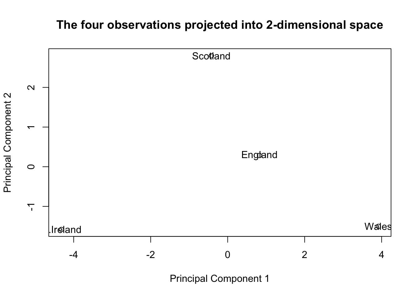
14.2.1.3 The BiPlot
Now we can also view our original variable axes projected down onto that same space!
biplot(pca$x,pca$rotation, cex = c(1.5, 1), col = c('black','red'))#, 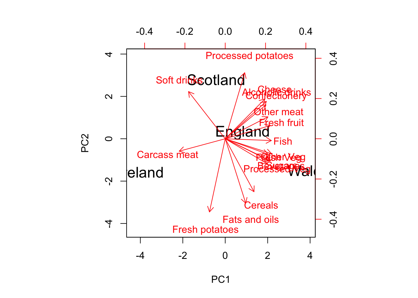
Figure 14.3: BiPlot: The observations and variables projected onto the same plane.
# xlim = c(-0.8,0.8), ylim = c(-0.6,0.7))14.2.1.4 Formatting the biplot for readability
I will soon introduce the autoplot() function from the ggfortify package, but for now I just want to show you that you can specify which variables (and observations) to include in the biplot by directly specifying the loadings matrix and scores matrix of interest in the biplot function:
desired.variables = c(2,4,6,8,10)
biplot(pca$x, pca$rotation[desired.variables,1:2], cex = c(1.5, 1),
       col = c('black','red'), xlim = c(-6,5), ylim = c(-4,4))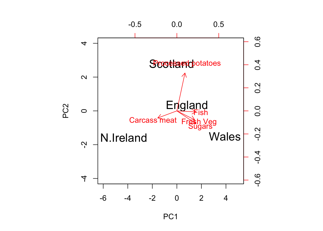
Figure 14.4: Specify a Subset of Variables/Observations to Include in the Biplot
14.2.1.5 What are all these axes?
Those numbers relate to the scores on PC1 and PC2 (sometimes normalized so that each new variable has variance 1 - and sometimes not) and the loadings on PC1 and PC2 (sometimes normalized so that each variable vector is a unit vector - and sometimes scaled by the eigenvalues or square roots of the eigenvalues in some fashion).
Generally, I’ve rarely found it useful to hunt down how each package is rendering the axes the biplot, as they should be providing the same information regardless of the scale of the numbers on the axes. We don’t actually use those numbers to help us draw conclusions. We use the directions of the arrows and the layout of the points in reference to those direction arrows.
vmax = varimax(pca$rotation[,1:2])
new.scores = pca$x[,1:2] %*% vmax$rotmat

biplot(new.scores, vmax$loadings[,1:2],
       # xlim=c(-60,60),
       # ylim=c(-60,60),
       cex = c(1.5, 1),
       xlab = 'Rotated Axis 1',
       ylab = 'Rotated Axis 2')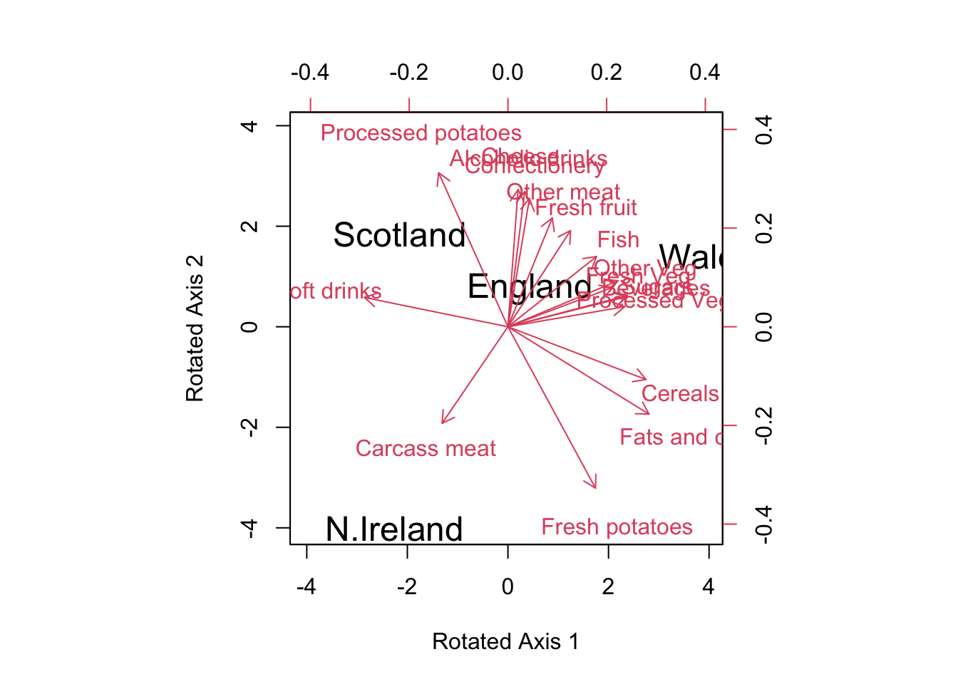
Figure 14.5: Biplot with Rotated Loadings
vmax$loadings[,1:2]## PC1 PC2
## Cheese 0.02571143 0.34751491
## Carcass meat -0.16660468 -0.24450375
## Other meat 0.11243721 0.27569481
## Fish 0.22437069 0.17788300
## Fats and oils 0.35728064 -0.22128124
## Sugars 0.30247003 0.07908986
## Fresh potatoes 0.22174898 -0.40880955
## Fresh Veg 0.26432097 0.09953752
## Other Veg 0.27836185 0.11640174
## Processed potatoes -0.17545152 0.39011648
## Processed Veg 0.29583164 0.05084727
## Fresh fruit 0.15852128 0.24360131
## Cereals 0.34963293 -0.13363398
## Beverages 0.30030152 0.07604823
## Soft drinks -0.36374762 0.07438738
## Alcoholic drinks 0.04243636 0.34240944
## Confectionery 0.05450175 0.3247482114.3 FIFA Soccer Players
14.3.0.1 Explore the Data
We begin by loading in the data and taking a quick look at the variables that we’ll be using in our PCA for this exercise. You may need to install the packages from the following library() statements.
library(reshape2) #melt correlation matrix into 3 columns
library(ggplot2) #correlation heatmap
library(ggfortify) #autoplot bi-plot
library(viridis) # magma palette
## Loading required package: viridisLitelibrary(plotrix) # color.legendNow we’ll read the data directly from the web, take a peek at the first 5 rows, and explore some summary statistics.
##                Name Age                                           Photo
## 1 Cristiano Ronaldo  32  https://cdn.sofifa.org/48/18/players/20801.png
## 2          L. Messi  30 https://cdn.sofifa.org/48/18/players/158023.png
## 3            Neymar  25 https://cdn.sofifa.org/48/18/players/190871.png
## 4         L. Suárez  30 https://cdn.sofifa.org/48/18/players/176580.png
## 5          M. Neuer  31 https://cdn.sofifa.org/48/18/players/167495.png
## 6    R. Lewandowski  28 https://cdn.sofifa.org/48/18/players/188545.png
##   Nationality                                Flag Overall Potential
## 1    Portugal https://cdn.sofifa.org/flags/38.png      94        94
## 2   Argentina https://cdn.sofifa.org/flags/52.png      93        93
## 3      Brazil https://cdn.sofifa.org/flags/54.png      92        94
## 4     Uruguay https://cdn.sofifa.org/flags/60.png      92        92
## 5     Germany https://cdn.sofifa.org/flags/21.png      92        92
## 6      Poland https://cdn.sofifa.org/flags/37.png      91        91
##                  Club                                  Club.Logo  Value  Wage
## 1      Real Madrid CF https://cdn.sofifa.org/24/18/teams/243.png €95.5M €565K
## 2        FC Barcelona https://cdn.sofifa.org/24/18/teams/241.png  €105M €565K
## 3 Paris Saint-Germain  https://cdn.sofifa.org/24/18/teams/73.png  €123M €280K
## 4        FC Barcelona https://cdn.sofifa.org/24/18/teams/241.png   €97M €510K
## 5    FC Bayern Munich  https://cdn.sofifa.org/24/18/teams/21.png   €61M €230K
## 6    FC Bayern Munich  https://cdn.sofifa.org/24/18/teams/21.png   €92M €355K
##   Special Acceleration Aggression Agility Balance Ball.control Composure
## 1    2228           89         63      89      63           93        95
## 2    2154           92         48      90      95           95        96
## 3    2100           94         56      96      82           95        92
## 4    2291           88         78      86      60           91        83
## 5    1493           58         29      52      35           48        70
## 6    2143           79         80      78      80           89        87
##   Crossing Curve Dribbling Finishing Free.kick.accuracy GK.diving GK.handling
## 1       85    81        91        94                 76         7          11
## 2       77    89        97        95                 90         6          11
## 3       75    81        96        89                 84         9           9
## 4       77    86        86        94                 84        27          25
## 5       15    14        30        13                 11        91          90
## 6       62    77        85        91                 84        15           6
##   GK.kicking GK.positioning GK.reflexes Heading.accuracy Interceptions Jumping
## 1         15             14          11               88            29      95
## 2         15             14           8               71            22      68
## 3         15             15          11               62            36      61
## 4         31             33          37               77            41      69
## 5         95             91          89               25            30      78
## 6         12              8          10               85            39      84
##   Long.passing Long.shots Marking Penalties Positioning Reactions Short.passing
## 1           77         92      22        85          95        96            83
## 2           87         88      13        74          93        95            88
## 3           75         77      21        81          90        88            81
## 4           64         86      30        85          92        93            83
## 5           59         16      10        47          12        85            55
## 6           65         83      25        81          91        91            83
##   Shot.power Sliding.tackle Sprint.speed Stamina Standing.tackle Strength
## 1         94             23           91      92              31       80
## 2         85             26           87      73              28       59
## 3         80             33           90      78              24       53
## 4         87             38           77      89              45       80
## 5         25             11           61      44              10       83
## 6         88             19           83      79              42       84
##   Vision Volleys position
## 1     85      88        1
## 2     90      85        1
## 3     80      83        1
## 4     84      88        1
## 5     70      11        4
## 6     78      87        1
## Acceleration Aggression Agility Balance Ball.control
## Min. :11.00 Min. :11.00 Min. :14.00 Min. :11.00 Min. : 8
## 1st Qu.:56.00 1st Qu.:43.00 1st Qu.:55.00 1st Qu.:56.00 1st Qu.:53
## Median :67.00 Median :58.00 Median :65.00 Median :66.00 Median :62
## Mean :64.48 Mean :55.74 Mean :63.25 Mean :63.76 Mean :58
## 3rd Qu.:75.00 3rd Qu.:69.00 3rd Qu.:74.00 3rd Qu.:74.00 3rd Qu.:69
## Max. :96.00 Max. :96.00 Max. :96.00 Max. :96.00 Max. :95
## Composure Crossing Curve Dribbling Finishing
## Min. : 5.00 Min. : 5.0 Min. : 6.0 Min. : 2.00 Min. : 2.00
## 1st Qu.:51.00 1st Qu.:37.0 1st Qu.:34.0 1st Qu.:48.00 1st Qu.:29.00
## Median :60.00 Median :54.0 Median :48.0 Median :60.00 Median :48.00
## Mean :57.82 Mean :49.7 Mean :47.2 Mean :54.94 Mean :45.18
## 3rd Qu.:67.00 3rd Qu.:64.0 3rd Qu.:62.0 3rd Qu.:68.00 3rd Qu.:61.00
## Max. :96.00 Max. :91.0 Max. :92.0 Max. :97.00 Max. :95.00
## Free.kick.accuracy GK.diving GK.handling GK.kicking
## Min. : 4.00 Min. : 1.00 Min. : 1.00 Min. : 1.00
## 1st Qu.:31.00 1st Qu.: 8.00 1st Qu.: 8.00 1st Qu.: 8.00
## Median :42.00 Median :11.00 Median :11.00 Median :11.00
## Mean :43.08 Mean :16.78 Mean :16.55 Mean :16.42
## 3rd Qu.:57.00 3rd Qu.:14.00 3rd Qu.:14.00 3rd Qu.:14.00
## Max. :93.00 Max. :91.00 Max. :91.00 Max. :95.00
## GK.positioning GK.reflexes Heading.accuracy Interceptions
## Min. : 1.00 Min. : 1.00 Min. : 4.00 Min. : 4.00
## 1st Qu.: 8.00 1st Qu.: 8.00 1st Qu.:44.00 1st Qu.:26.00
## Median :11.00 Median :11.00 Median :55.00 Median :52.00
## Mean :16.54 Mean :16.91 Mean :52.26 Mean :46.53
## 3rd Qu.:14.00 3rd Qu.:14.00 3rd Qu.:64.00 3rd Qu.:64.00
## Max. :91.00 Max. :90.00 Max. :94.00 Max. :92.00
## Jumping Long.passing Long.shots Marking
## Min. :15.00 Min. : 7.00 Min. : 3.00 Min. : 4.00
## 1st Qu.:58.00 1st Qu.:42.00 1st Qu.:32.00 1st Qu.:22.00
## Median :66.00 Median :56.00 Median :51.00 Median :48.00
## Mean :64.84 Mean :52.37 Mean :47.11 Mean :44.09
## 3rd Qu.:73.00 3rd Qu.:64.00 3rd Qu.:62.00 3rd Qu.:63.00
## Max. :95.00 Max. :93.00 Max. :92.00 Max. :92.00
## Penalties Positioning Reactions Short.passing
## Min. : 5.00 Min. : 2.00 Min. :28.00 Min. :10.00
## 1st Qu.:39.00 1st Qu.:38.00 1st Qu.:55.00 1st Qu.:53.00
## Median :50.00 Median :54.00 Median :62.00 Median :62.00
## Mean :48.92 Mean :49.53 Mean :61.85 Mean :58.22
## 3rd Qu.:61.00 3rd Qu.:64.00 3rd Qu.:68.00 3rd Qu.:68.00
## Max. :92.00 Max. :95.00 Max. :96.00 Max. :92.00
## Shot.power Sliding.tackle Sprint.speed Stamina
## Min. : 3.00 Min. : 4.00 Min. :11.00 Min. :12.00
## 1st Qu.:46.00 1st Qu.:24.00 1st Qu.:57.00 1st Qu.:56.00
## Median :59.00 Median :52.00 Median :67.00 Median :66.00
## Mean :55.57 Mean :45.56 Mean :64.72 Mean :63.13
## 3rd Qu.:68.00 3rd Qu.:64.00 3rd Qu.:75.00 3rd Qu.:74.00
## Max. :94.00 Max. :91.00 Max. :96.00 Max. :95.00
## Standing.tackle Strength Vision Volleys
## Min. : 4.00 Min. :20.00 Min. :10.00 Min. : 4.00
## 1st Qu.:26.00 1st Qu.:58.00 1st Qu.:43.00 1st Qu.:30.00
## Median :54.00 Median :66.00 Median :54.00 Median :44.00
## Mean :47.41 Mean :65.24 Mean :52.93 Mean :43.13
## 3rd Qu.:66.00 3rd Qu.:74.00 3rd Qu.:64.00 3rd Qu.:57.00
## Max. :92.00 Max. :98.00 Max. :94.00 Max. :91.00These variables are scores on the scale of [0,100] that measure 34 key abilities of soccer players. No player has ever earned a score of 100 on any of these attributes - no player is perfect!
It would be natural to assume some correlation between these variables and indeed, we see lots of it in the following heatmap visualization of the correlation matrix.
cor.matrix = cor(fifa[,13:46])
cor.matrix = melt(cor.matrix)
ggplot(data = cor.matrix, aes(x=Var1, y=Var2, fill=value)) +
  geom_tile(color = "white")+
  scale_fill_gradient2(low = "blue", high = "red", mid = "white",
   midpoint = 0, limit = c(-1,1), space = "Lab",
    name="Correlation") +  theme_minimal()+
      theme(axis.title.x = element_blank(),axis.title.y = element_blank(),
            axis.text.x = element_text(angle = 45, vjust = 1,
        size = 9, hjust = 1))+coord_fixed()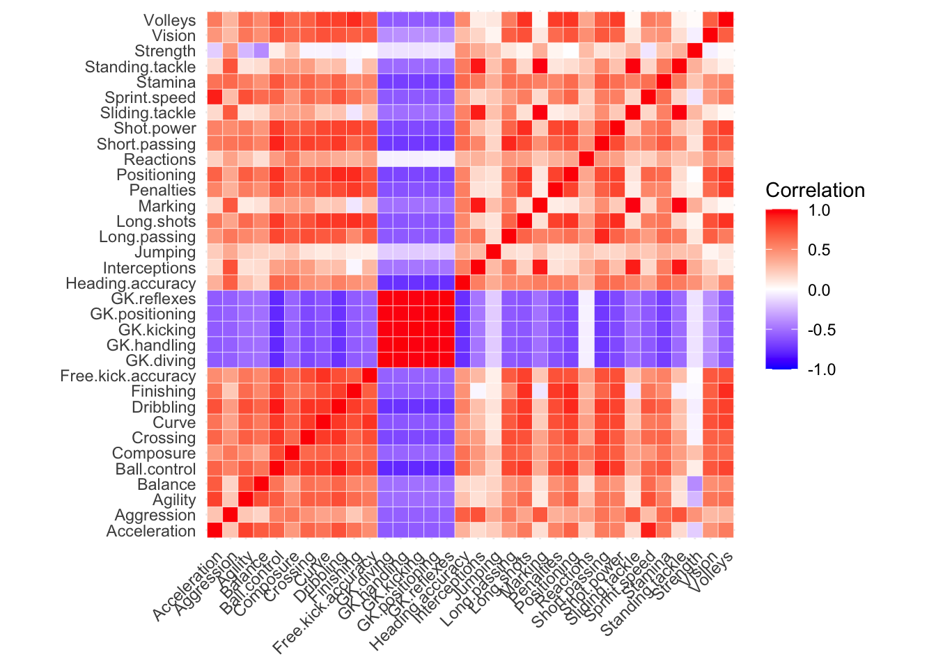
Figure 14.6: Heatmap of correlation matrix for 34 variables of interest
What jumps out right away are the “GK” (Goal Keeping) abilities - these attributes have very strong positive correlation with one another and negative correlation with the other abilities. After all, goal keepers are not traditionally well known for their dribbling, passing, and finishing abilities!
Outside of that, we see a lot of red in this correlation matrix – many attributes share a lot of information. This is the type of situation where PCA shines.
14.3.0.2 Principal Components Analysis
Let’s take a look at the principal components analysis. Since the variables are on the same scale, I’ll start with covariance PCA (the default in R’s prcomp() function).
fifa.pca = prcomp(fifa[,13:46] )We can then print the summary of variance explained and the loadings on the first 3 components:
summary(fifa.pca)## Importance of components:
## PC1 PC2 PC3 PC4 PC5 PC6
## Standard deviation 74.8371 43.5787 23.28767 20.58146 16.12477 10.71539
## Proportion of Variance 0.5647 0.1915 0.05468 0.04271 0.02621 0.01158
## Cumulative Proportion 0.5647 0.7561 0.81081 0.85352 0.87973 0.89131
## PC7 PC8 PC9 PC10 PC11 PC12 PC13
## Standard deviation 10.17785 9.11852 8.98065 8.5082 8.41550 7.93741 7.15935
## Proportion of Variance 0.01044 0.00838 0.00813 0.0073 0.00714 0.00635 0.00517
## Cumulative Proportion 0.90175 0.91013 0.91827 0.9256 0.93270 0.93906 0.94422
## PC14 PC15 PC16 PC17 PC18 PC19 PC20
## Standard deviation 7.06502 6.68497 6.56406 6.50459 6.22369 6.08812 6.00578
## Proportion of Variance 0.00503 0.00451 0.00434 0.00427 0.00391 0.00374 0.00364
## Cumulative Proportion 0.94926 0.95376 0.95811 0.96237 0.96628 0.97001 0.97365
## PC21 PC22 PC23 PC24 PC25 PC26 PC27
## Standard deviation 5.91320 5.66946 5.45018 5.15051 4.86761 4.34786 4.1098
## Proportion of Variance 0.00353 0.00324 0.00299 0.00267 0.00239 0.00191 0.0017
## Cumulative Proportion 0.97718 0.98042 0.98341 0.98609 0.98848 0.99038 0.9921
## PC28 PC29 PC30 PC31 PC32 PC33 PC34
## Standard deviation 4.05716 3.46035 3.37936 3.31179 3.1429 3.01667 2.95098
## Proportion of Variance 0.00166 0.00121 0.00115 0.00111 0.0010 0.00092 0.00088
## Cumulative Proportion 0.99374 0.99495 0.99610 0.99721 0.9982 0.99912 1.00000fifa.pca$rotation[,1:3]## PC1 PC2 PC3
## Acceleration -0.13674335 0.0944478107 -0.141193842
## Aggression -0.15322857 -0.2030537953 0.105372978
## Agility -0.13598896 0.1196301737 -0.017763073
## Balance -0.11474980 0.0865672989 -0.072629834
## Ball.control -0.21256812 0.0585990154 0.038243802
## Composure -0.13288575 -0.0005635262 0.163887637
## Crossing -0.21347202 0.0458210228 0.124741235
## Curve -0.20656129 0.1254947094 0.180634730
## Dribbling -0.23090613 0.1259819707 -0.002905379
## Finishing -0.19431248 0.2534086437 0.006524693
## Free.kick.accuracy -0.18528508 0.0960404650 0.219976709
## GK.diving 0.20757999 0.0480952942 0.326161934
## GK.handling 0.19811125 0.0464542553 0.314165622
## GK.kicking 0.19261876 0.0456942190 0.304722126
## GK.positioning 0.19889113 0.0456384196 0.317850121
## GK.reflexes 0.21081755 0.0489895700 0.332751195
## Heading.accuracy -0.17218607 -0.1115416097 -0.125135161
## Interceptions -0.15038835 -0.3669025376 0.162064432
## Jumping -0.03805419 -0.0579221746 0.012263523
## Long.passing -0.16849827 -0.0435009943 0.224584171
## Long.shots -0.21415526 0.1677851237 0.157466462
## Marking -0.14863254 -0.4076616902 0.078298039
## Penalties -0.16328049 0.1407803994 0.024403976
## Positioning -0.22053959 0.1797895382 0.020734699
## Reactions -0.04780774 0.0001844959 0.250247098
## Short.passing -0.18176636 -0.0033124240 0.118611543
## Shot.power -0.19592137 0.0989340925 0.101707386
## Sliding.tackle -0.14977558 -0.4024030355 0.069945935
## Sprint.speed -0.13387287 0.0804847541 -0.146049405
## Stamina -0.17231648 -0.0634639786 -0.016509650
## Standing.tackle -0.15992073 -0.4039763876 0.086418583
## Strength -0.02186264 -0.1151018222 0.096053864
## Vision -0.13027169 0.1152237536 0.260985686
## Volleys -0.18465028 0.1888480712 0.076974579It’s clear we can capture a large amount of the variance in this data with just a few components. In fact just 2 components yield 76% of the variance!
Now let’s look at some projections of the players onto those 2 principal components. The scores are located in the fifa.pca$x matrix.
plot(fifa.pca$x[,1],fifa.pca$x[,2], col=alpha(c('red','blue','green','black')[as.factor(fifa$position)],0.4), pch=16, xlab = 'Principal Component 1', ylab='Principal Component 2', main = 'Projection of Players onto 2 PCs, Colored by Position')
legend(125,-45, c('Forward','Defense','Midfield','GoalKeeper'), c('red','blue','green','black'), bty = 'n', cex=1.1)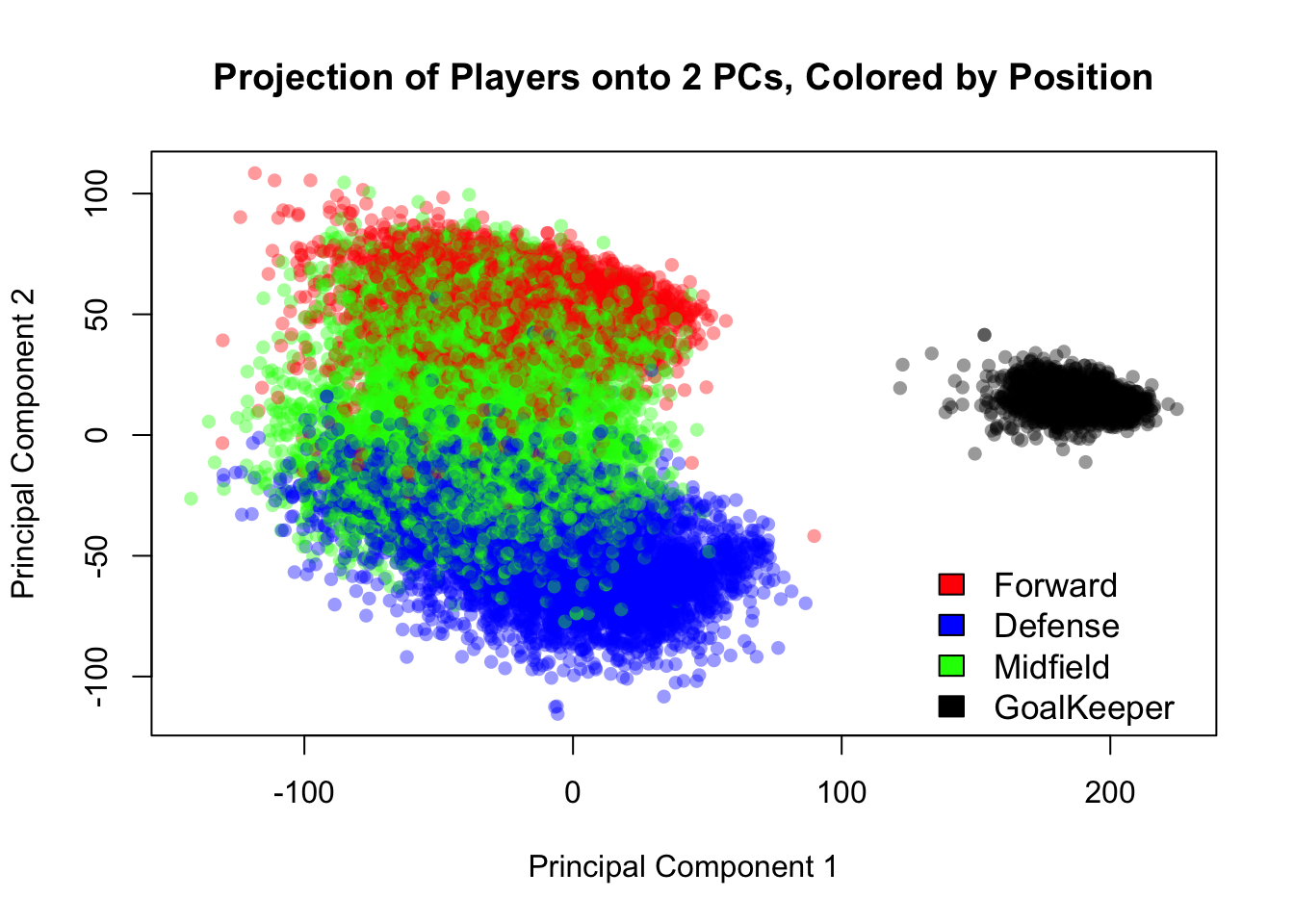
Figure 14.7: Projection of the FIFA players’ skill data into 2 dimensions. Player positions are evident.
The plot easily separates the field players from the goal keepers, and the forwards from the defenders. As one might expect, midfielders are sandwiched by the forwards and defenders, as they play both roles on the field. The labeling of player position was imperfect and done using a list of the players’ preferred positions, and it’s likely we are seeing that in some of the players labeled as midfielders that appear above the cloud of red points.
We can also attempt a 3-dimensional projection of this data:
library(plotly)
library(processx)
colors=alpha(c('red','blue','green','black')[as.factor(fifa$position)],0.4)
graph = plot_ly(x = fifa.pca$x[,1],
                y = fifa.pca$x[,2],
                z= fifa.pca$x[,3],
                type='scatter3d',
                mode="markers",
                marker = list(color=colors))
graph
Figure 14.8: Projection of the FIFA players’ skill data into 3 dimensions. Player positions are evident.
14.3.0.3 The BiPlot
BiPlots can be tricky when we have so much data and so many variables. As you will see, the default image leaves much to be desired, and will motivate our move to the ggfortify library to use the autoplot() function. The image takes too long to render and is practically unreadable with the whole dataset, so I demonstrate the default biplot() function with a sample of the observations.
biplot(fifa.pca$x[sample(1:16501,2000),],fifa.pca$rotation[,1:2], cex=0.5, arrow.len = 0.1)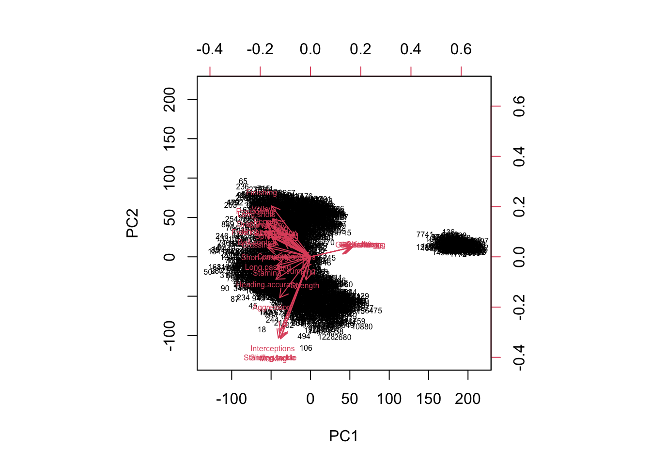
Figure 14.9: The default biplot function leaves much to be desired here
The autoplot function uses the `ggplot2``` package and is superior when we have more data.
autoplot(fifa.pca, data = fifa,
         colour = alpha(c('red','blue','green','orange')[as.factor(fifa$pos)],0.4),
         loadings = TRUE, loadings.colour = 'black',
         loadings.label = TRUE, loadings.label.size = 3.5, loadings.label.alpha = 1,
         loadings.label.fontface='bold',
         loadings.label.colour = 'black',
         loadings.label.repel=T)
## Warning: `select_()` was deprecated in dplyr 0.7.0.
## Please use `select()` instead.## Warning in if (value %in% columns) {: the condition has length > 1 and only the
## first element will be used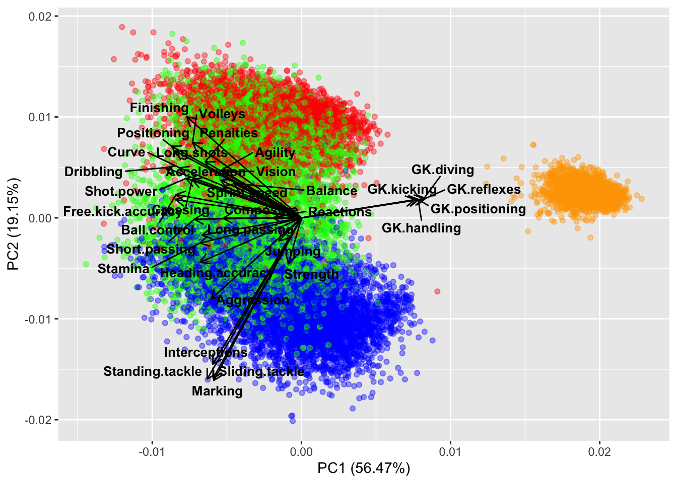
Figure 14.10: The autoplot() biplot has many more options for readability.
Many expected conclusions can be drawn from this biplot. The defenders tend to have stronger skills of interception, slide tackling, standing tackling, and marking, while forwards are generally stronger when it comes to finishing, long.shots, volleys, agility etc. Midfielders are likely to be stronger with crossing, passing, ball.control, and stamina.
14.3.0.4 Further Exploration
Let’s see what happens if we color by the variable ‘overall’ which is designed to rank a player’s overall quality of play.
palette(alpha(magma(100),0.6))

plot(fifa.pca$x[,1],fifa.pca$x[,2], col=fifa$Overall,pch=16, xlab = 'Principal Component 1', ylab='Principal Component 2')

color.legend(130,-100,220,-90,seq(0,100,50),alpha(magma(100),0.6),gradient="x")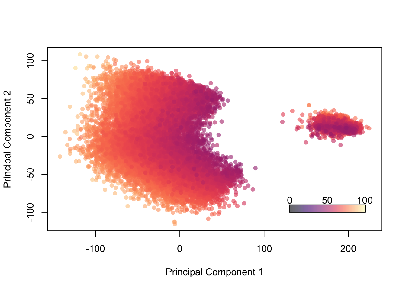
Figure 14.11: Projection of Players onto 2 PCs, Colored by “Overall” Ability
We can attempt to label some of the outliers, too. First, we’ll look at the 0.001 and 0.999 quantiles to get a sense of what coordinates we want to highlight. Then we’ll label any players outside of those bounds and surely find some familiar names.
# This first chunk is identical to the chunk above. I have to reproduce the plot to label it.
palette(alpha(magma(100),0.6))
plot(fifa.pca$x[,1], fifa.pca$x[,2], col=fifa$Overall,pch=16, xlab = 'Principal Component 1', ylab='Principal Component 2',
     xlim=c(-175,250), ylim = c(-150,150))
color.legend(130,-100,220,-90,seq(0,100,50),alpha(magma(100),0.6),gradient="x")

# Identify quantiles (high/low) for each PC
(quant1h = quantile(fifa.pca$x[,1],0.9997))
## 99.97%
## 215.4003(quant1l = quantile(fifa.pca$x[,1],0.0003))## 0.03%
## -130.1493(quant2h = quantile(fifa.pca$x[,2],0.9997))## 99.97%
## 100.208(quant2l = quantile(fifa.pca$x[,2],0.0003))## 0.03%
## -101.8846# Next I create a logical vector which identifies the outliers
# (i.e. TRUE = outlier, FALSE = not outlier)
outliers = fifa.pca$x[,1] > quant1h | fifa.pca$x[,1] < quant1l |
fifa.pca$x[,2] > quant2h | fifa.pca$x[,2] < quant2l
# Here I label them by name, jittering the coordinates of the text so it's more readable
text(jitter(fifa.pca$x[outliers,1],factor=1), jitter(fifa.pca$x[outliers,2],factor=600), fifa$Name[outliers], cex=0.7)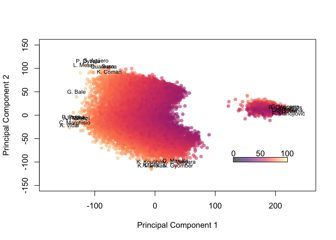
What about by wage? First we need to convert their salary, denominated in Euros, to a numeric variable.
# First, observe the problem with the Wage column as it stands
head(fifa$Wage)
## [1] "€565K" "€565K" "€280K" "€510K" "€230K" "€355K"# Use regular expressions to remove the Euro sign and K from the wage column
# then covert to numeric
fifa$Wage = as.numeric(gsub('[€K]', '', fifa$Wage))
# new data:
head(fifa$Wage)## [1] 565 565 280 510 230 355palette(alpha(magma(100),0.6))
plot(fifa.pca$x[,1], fifa.pca$x[,2], col=fifa$Wage,pch=16, xlab = 'Principal Component 1', ylab='Principal Component 2')
color.legend(130,-100,220,-90,c(min(fifa$Wage),max(fifa$Wage)),alpha(magma(100),0.6),gradient="x")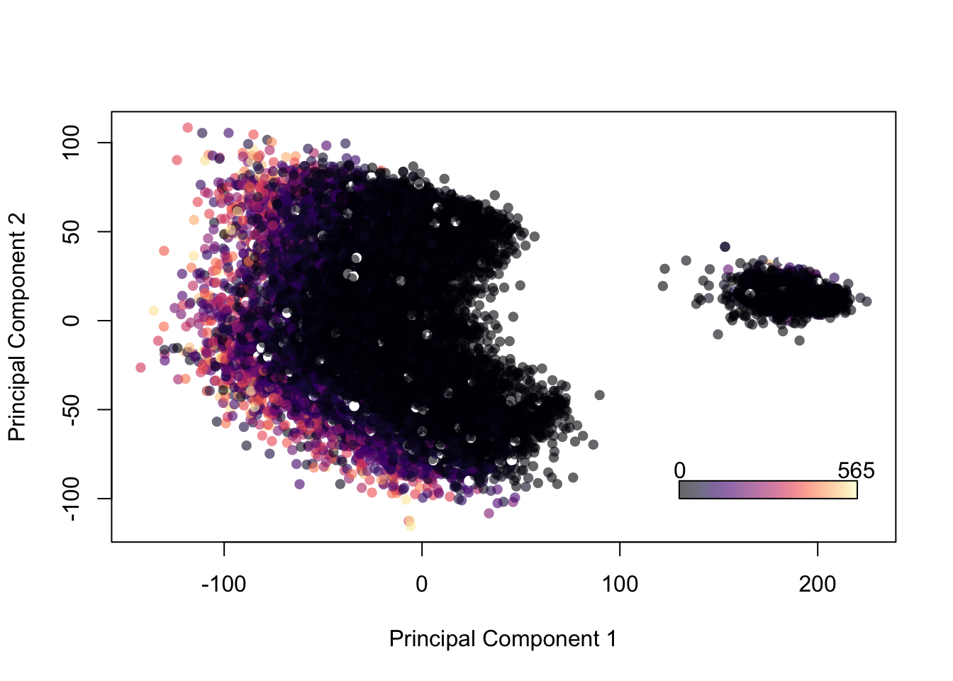
Figure 14.12: Projection of Players onto 2 Principal Components, Colored by Wage
14.3.0.5 Rotations of Principal Components
We might be able to align our axes more squarely with groups of original variables that are strongly correlated and tell a story. Perhaps we might be able to find latent variables that indicate the position specific ability of players. Let’s see what falls out after varimax and quartimax rotation. Recall that in order to employ rotations, we have to first decide on a number of components. A quick look at a screeplot or cumulative proportion variance explained should help to that aim.
plot(cumsum(fifa.pca$sdev^2)/sum(fifa.pca$sdev^2),
     type = 'b',
     cex=.75,
     xlab = "# of components",
     ylab = "% variance explained")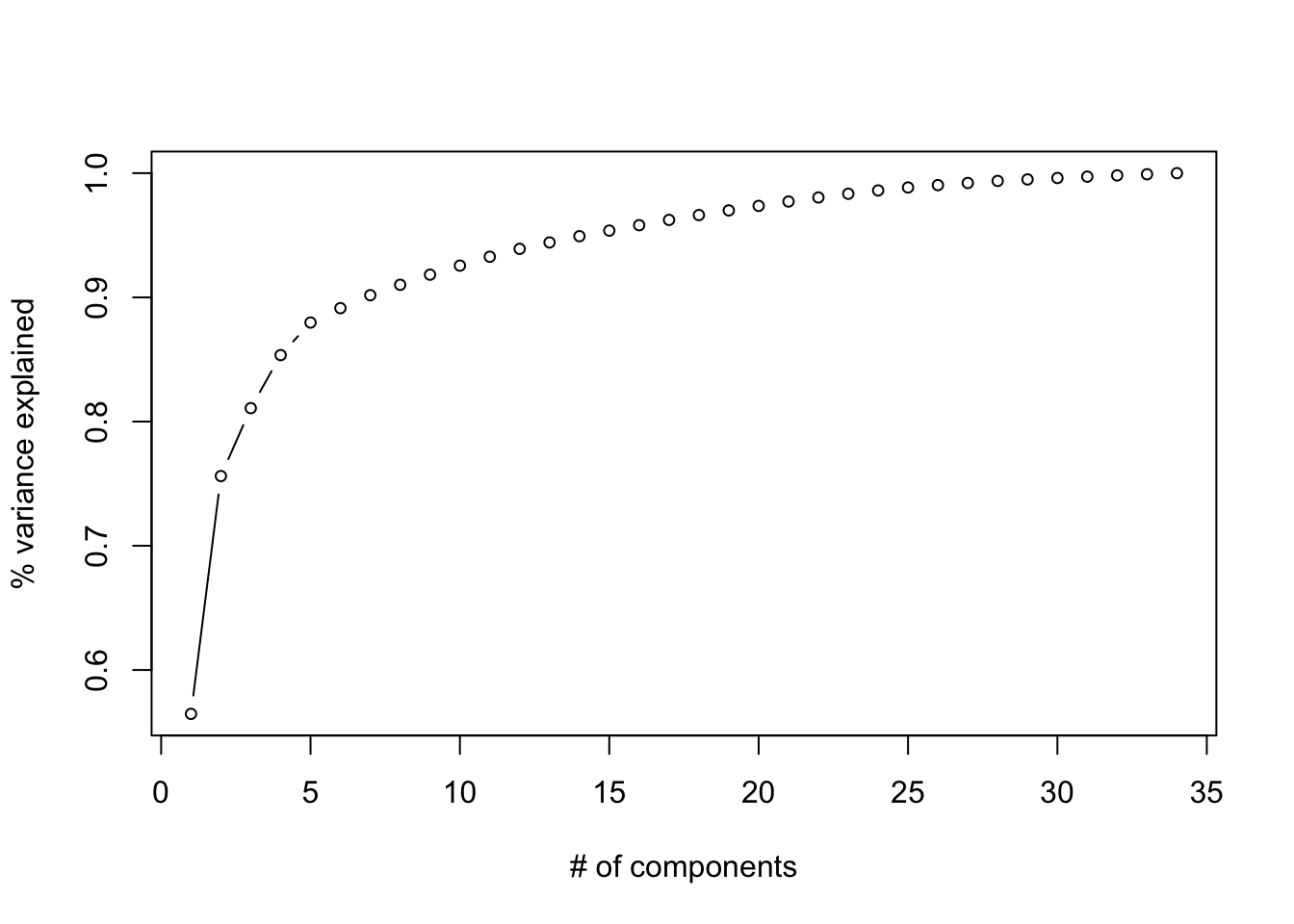
Figure 14.13: Cumulative proportion of variance explained by rank of the decomposition (i.e. the number of components)
Let’s use 3 components, since the marginal benefit of using additional components seems small. Once we rotate the loadings, we can try to use a heatmap to visualize what they might represent.
vmax = varimax(fifa.pca$rotation[,1:3])
loadings = fifa.pca$rotation[,1:3]%*%vmax$rotmat
melt.loadings = melt(loadings)
ggplot(data = melt.loadings, aes(x=Var2, y=Var1, fill=value)) +
  geom_tile(color = "white")+
  scale_fill_gradient2(low = "blue", high = "red", mid = "white",
   midpoint = 0, limit = c(-1,1))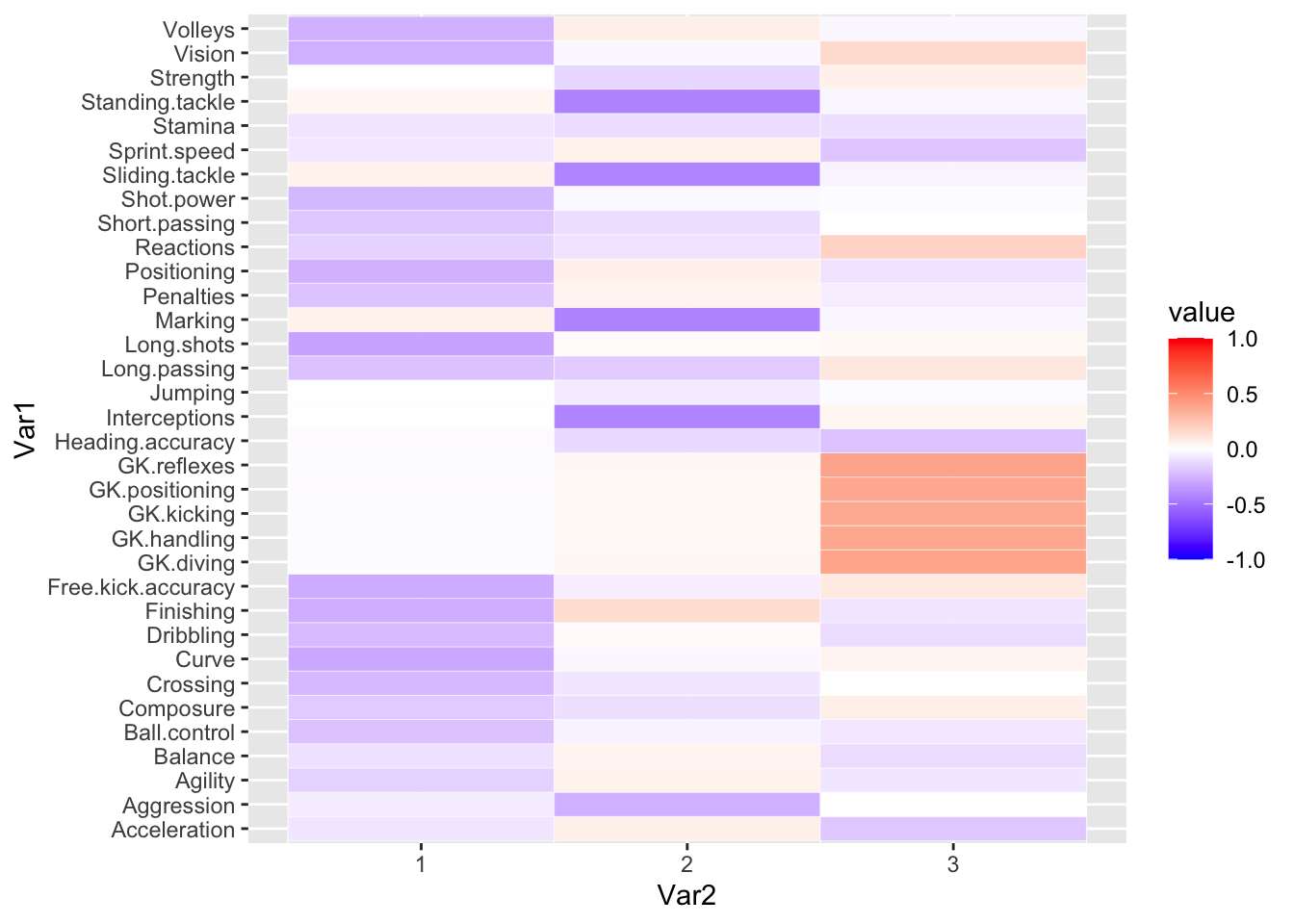
14.4 Cancer Genetics
Read in the data. The load() function reads in a dataset that has 20532 columns and may take some time. You may want to save and clear your environment (or open a new RStudio window) if you have other work open.
load('LAdata/geneCancerUCI.RData')
table(cancerlabels$Class)
##
## BRCA COAD KIRC LUAD PRAD
## 300 78 146 141 136Original Source: The cancer genome atlas pan-cancer analysis project
- BRCA = Breast Invasive Carcinoma
- COAD = Colon Adenocarcinoma
- KIRC = Kidney Renal clear cell Carcinoma
- LUAD = Lung Adenocarcinoma
- PRAD = Prostate Adenocarcinoma
We are going to want to plot the data points according to their different classification labels. We should pick out a nice color palette for categorical attributes. We chose to assign palette Dark2 but feel free to choose any categorical palette that attracts you in the code below!
library(RColorBrewer)
display.brewer.all()
palette(brewer.pal(n = 8, name = "Dark2"))
The first step is typically to explore the data. Obviously we can’t look at ALL the scatter plots of input variables. For the fun of it, let’s look at a few of these scatter plots which we’ll pick at random. First pick two column numbers at random, then draw the plot, coloring by the label. You could repeat this chunk several times to explore different combinations. Can you find one that does a good job of separating any of the types of cancer?
par(mfrow=c(2,3))
for(i in 1:6){
randomColumns = sample(2:20532,2)
plot(cancer[,randomColumns],col = cancerlabels$Class)
}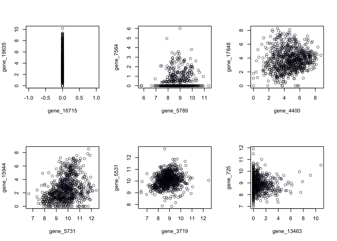
Figure 14.14: Random 2-Dimensional Projections of Cancer Data
To restore our plot window from that 3-by-2 grid, we run dev.off()
dev.off()## null device
## 114.4.1 Computing the PCA
The function is the one I most often recommend for reasonably sized principal component calculations in R. This function returns a list with class “prcomp” containing the following components (from help prcomp):
- : the standard deviations of the principal components (i.e., the square roots of the eigenvalues of the covariance/correlation matrix, though the calculation is actually done with the singular values of the data matrix).
- : the matrix of variable loadings (i.e., a matrix whose columns contain the eigenvectors). The function princomp returns this in the element loadings.
- : if retx is true the value of the rotated data (i.e. the scores) (the centred (and scaled if requested) data multiplied by the rotation matrix) is returned. Hence, cov(x) is the diagonal matrix \(diag(sdev^2)\). For the formula method, napredict() is applied to handle the treatment of values omitted by the na.action.
- : the centering and scaling used, or FALSE.
The option inside the function instructs the program to use correlation PCA. The default is covariance PCA.
Now let’s compute the first three principal components and examine the data projected onto the first 2 axes. We can then look in 3 dimensions.
pcaOut = prcomp(cancer,rank = 3, scale = F)plot(pcaOut$x[,1], pcaOut$x[,2],
col = cancerlabels$Class,
xlab = "Principal Component 1",
ylab = "Principal Component 2",
main = 'Genetic Samples Projected into 2-dimensions \n using COVARIANCE PCA')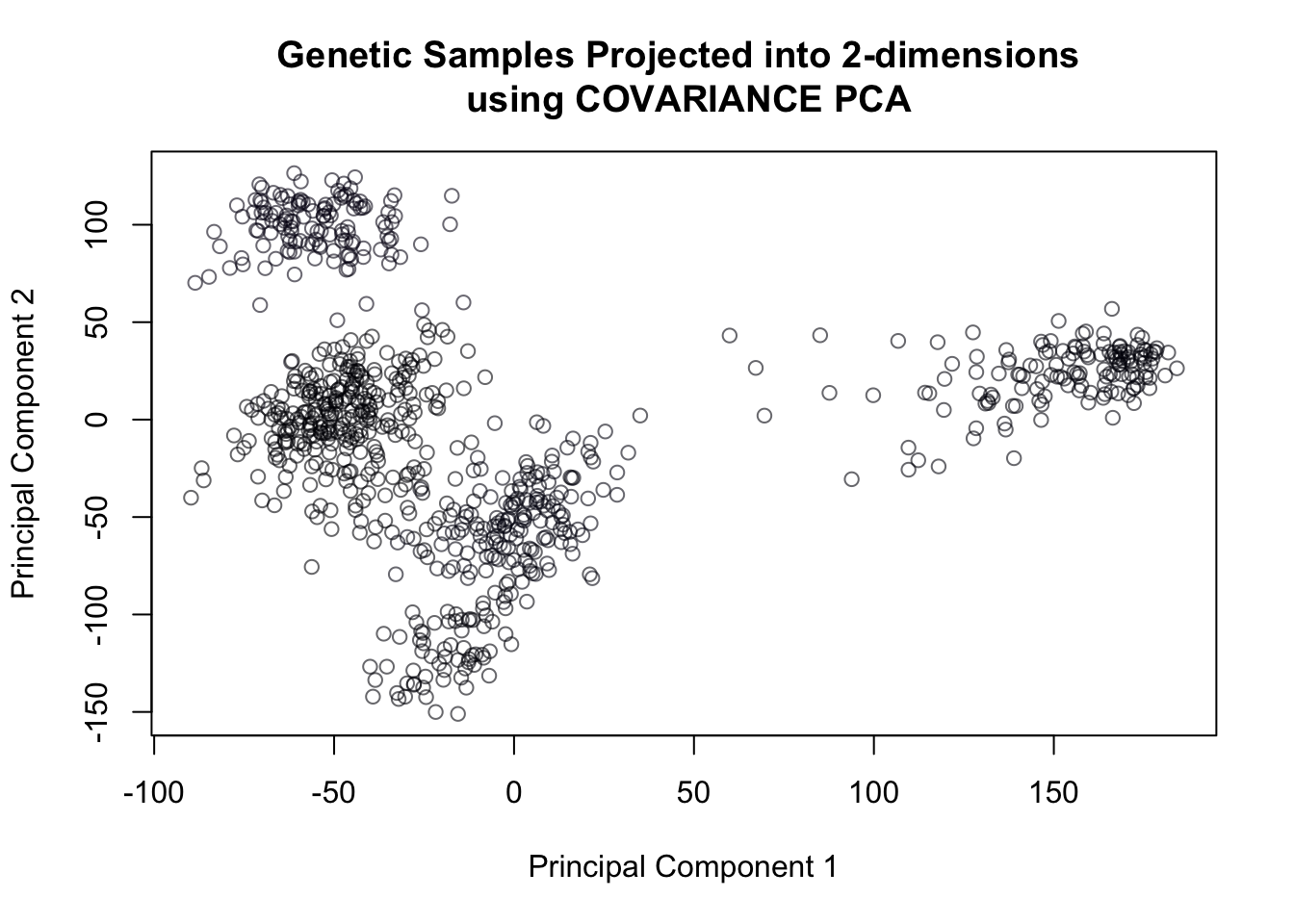
Figure 14.15: Covariance PCA of genetic data
14.4.2 3D plot with package
Make sure the plotly package is installed for the 3d plot. To get the plot points colored by group, we need to execute the following command that creates a vector of colors (specifying a color for each observation).
colors = factor(palette())
colors = colors[cancerlabels$Class]
table(colors, cancerlabels$Class)
##
## colors BRCA COAD KIRC LUAD PRAD
## #00000499 300 0 0 0 0
## #01010799 0 78 0 0 0
## #02020B99 0 0 146 0 0
## #03031199 0 0 0 141 0
## #05041799 0 0 0 0 136
## #07061C99 0 0 0 0 0
## #09072199 0 0 0 0 0
## #0C092699 0 0 0 0 0
## #0F0B2C99 0 0 0 0 0
## #120D3299 0 0 0 0 0
## #150E3799 0 0 0 0 0
## #180F3E99 0 0 0 0 0
## #1C104499 0 0 0 0 0
## #1F114A99 0 0 0 0 0
## #22115099 0 0 0 0 0
## #26125799 0 0 0 0 0
## #2A115D99 0 0 0 0 0
## #2F116399 0 0 0 0 0
## #33106899 0 0 0 0 0
## #38106C99 0 0 0 0 0
## #3C0F7199 0 0 0 0 0
## #400F7499 0 0 0 0 0
## #45107799 0 0 0 0 0
## #49107899 0 0 0 0 0
## #4E117B99 0 0 0 0 0
## #51127C99 0 0 0 0 0
## #56147D99 0 0 0 0 0
## #5A167E99 0 0 0 0 0
## #5D177F99 0 0 0 0 0
## #61198099 0 0 0 0 0
## #661A8099 0 0 0 0 0
## #6A1C8199 0 0 0 0 0
## #6D1D8199 0 0 0 0 0
## #721F8199 0 0 0 0 0
## #76218199 0 0 0 0 0
## #79228299 0 0 0 0 0
## #7D248299 0 0 0 0 0
## #82258199 0 0 0 0 0
## #86278199 0 0 0 0 0
## #8A298199 0 0 0 0 0
## #8E2A8199 0 0 0 0 0
## #922B8099 0 0 0 0 0
## #962C8099 0 0 0 0 0
## #9B2E7F99 0 0 0 0 0
## #9F2F7F99 0 0 0 0 0
## #A3307E99 0 0 0 0 0
## #A7317D99 0 0 0 0 0
## #AB337C99 0 0 0 0 0
## #AF357B99 0 0 0 0 0
## #B3367A99 0 0 0 0 0
## #B8377999 0 0 0 0 0
## #BC397899 0 0 0 0 0
## #C03A7699 0 0 0 0 0
## #C43C7599 0 0 0 0 0
## #C83E7399 0 0 0 0 0
## #CD407199 0 0 0 0 0
## #D0416F99 0 0 0 0 0
## #D5446D99 0 0 0 0 0
## #D8456C99 0 0 0 0 0
## #DC486999 0 0 0 0 0
## #DF4B6899 0 0 0 0 0
## #E34E6599 0 0 0 0 0
## #E6516399 0 0 0 0 0
## #E9556299 0 0 0 0 0
## #EC586099 0 0 0 0 0
## #EE5C5E99 0 0 0 0 0
## #F1605D99 0 0 0 0 0
## #F2655C99 0 0 0 0 0
## #F4695C99 0 0 0 0 0
## #F66D5C99 0 0 0 0 0
## #F7735C99 0 0 0 0 0
## #F9785D99 0 0 0 0 0
## #F97C5D99 0 0 0 0 0
## #FA815F99 0 0 0 0 0
## #FB866199 0 0 0 0 0
## #FC8A6299 0 0 0 0 0
## #FC906599 0 0 0 0 0
## #FCEFB199 0 0 0 0 0
## #FCF4B699 0 0 0 0 0
## #FCF8BA99 0 0 0 0 0
## #FCFDBF99 0 0 0 0 0
## #FD956799 0 0 0 0 0
## #FD9A6A99 0 0 0 0 0
## #FDDC9E99 0 0 0 0 0
## #FDE1A299 0 0 0 0 0
## #FDE5A799 0 0 0 0 0
## #FDEBAB99 0 0 0 0 0
## #FE9E6C99 0 0 0 0 0
## #FEA36F99 0 0 0 0 0
## #FEA87399 0 0 0 0 0
## #FEAC7699 0 0 0 0 0
## #FEB27A99 0 0 0 0 0
## #FEB67D99 0 0 0 0 0
## #FEBB8199 0 0 0 0 0
## #FEC08599 0 0 0 0 0
## #FEC48899 0 0 0 0 0
## #FEC98D99 0 0 0 0 0
## #FECD9099 0 0 0 0 0
## #FED39599 0 0 0 0 0
## #FED79999 0 0 0 0 0library(plotly)
graph = plot_ly(x = pcaOut$x[,1],
y = pcaOut$x[,2],
z= pcaOut$x[,3],
type='scatter3d',
mode="markers",
marker = list(color=colors))
graph14.4.3 3D plot with package
library(rgl)##
## Attaching package: 'rgl'## The following object is masked from 'package:plotrix':
##
## mtext3dknitr::knit_hooks$set(webgl = hook_webgl)Make sure the rgl package is installed for the 3d plot.
plot3d(x = pcaOut$x[,1],
       y = pcaOut$x[,2],
       z= pcaOut$x[,3],
       col = colors,
       xlab = "Principal Component 1",
       ylab = "Principal Component 2",
       zlab = "Principal Component 3")
You must enable Javascript to view this page properly.
14.4.4 Variance explained
Proportion of Variance explained by 2,3 components:
summary(pcaOut)## Importance of first k=3 (out of 801) components:
## PC1 PC2 PC3
## Standard deviation 75.7407 61.6805 58.57297
## Proportion of Variance 0.1584 0.1050 0.09472
## Cumulative Proportion 0.1584 0.2634 0.35815# Alternatively, if you had computed the ALL the principal components (omitted the rank=3 option) then
# you could directly compute the proportions of variance explained using what we know about the
# eigenvalues:
# sum(pcaOut$sdev[1:2]^2)/sum(pcaOut$sdev^2)
# sum(pcaOut$sdev[1:3]^2)/sum(pcaOut$sdev^2)14.4.5 Using Correlation PCA
The data involved in this exercise are actually on the same scale, and normalizing them may not be in your best interest because of this. However, it’s always a good idea to explore both decompositions if you have time.
pca.cor = prcomp(cancer, rank=3, scale =T)An error message! Cannot rescale a constant/zero column to unit variance. Solution: check for columns with zero variance and remove them. Then, re-check dimensions of the matrix to see how many columns we lost.
cancer = cancer[,apply(cancer, 2, sd)>0 ]
dim(cancer)
## [1] 801 20264Once we’ve taken care of those zero-variance columns, we can proceed to compute the correlation PCA:
pca.cor = prcomp(cancer, rank=3, scale =T)plot(pca.cor$x[,1], pca.cor$x[,2],
col = cancerlabels$Class,
xlab = "Principal Component 1",
ylab = "Principal Component 2",
main = 'Genetic Samples Projected into 2-dimensions \n using CORRELATION PCA')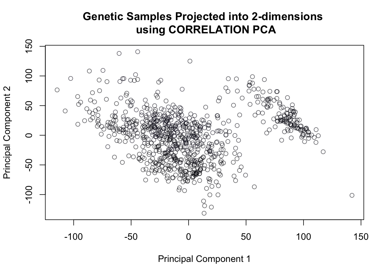
Figure 14.16: Correlation PCA of genetic data
And it’s clear just from the 2-dimensional projection that correlation PCA does not seem to work as well as covariance PCA when it comes to separating the 4 different types of cancer.
Indeed, we can confirm this from the proportion of variance explained, which is substantially lower than that of covariance PCA:
summary(pca.cor)## Importance of first k=3 (out of 801) components:
## PC1 PC2 PC3
## Standard deviation 46.2145 42.11838 39.7823
## Proportion of Variance 0.1054 0.08754 0.0781
## Cumulative Proportion 0.1054 0.19294 0.271014.4.6 Range standardization as an alternative to covariance PCA
We can also put all the variables on a scale of 0 to 1 if we’re concerned about issues with scale (in this case, scale wasn’t an issue - but the following approach still might be provide interesting projections in some datasets). This transformation would be as follows for each variable \(\mathbf{x}\): \[\frac{\mathbf{x} - \min(\mathbf{x})}{\max(\mathbf{x})-\min(\mathbf{x})}\]
cancer = cancer[,apply(cancer,2,sd)>0]

min = apply(cancer,2,min)
range =   apply(cancer,2, function(x){max(x)-min(x)})
minmax.cancer=scale(cancer,center=min,scale=range)
Then we can compute the covariance PCA of that range-standardized data without concern:
minmax.pca = prcomp(minmax.cancer, rank=3, scale=F ) plot(minmax.pca$x[,1],minmax.pca$x[,2],col = cancerlabels$Class, xlab = "Principal Component 1", ylab = "Principal Component 2")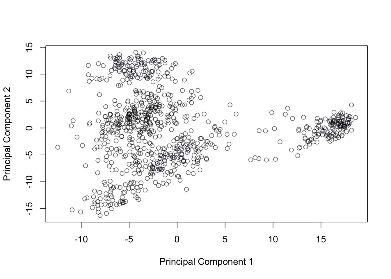
Figure 14.17: Covariance PCA of range standardized genetic data