Chapter 2 Matrix Arithmetic

2.1 Matrix Addition, Subtraction, and Scalar Multiplication

Addition, subtraction, and scalar multiplication are the only operations which act element-wise on matrices - they are performed in a way you might expect given your previous studies.

Definition 2.1 (Addition, Subtraction, and Scalar Multiplication) Two matrices can be added or subtracted only when they have the same dimensions. If \(\mathbf{A}\) and \(\mathbf{B}\) are both \(m\times n\) matrices then the (i,j) element of the sum (or difference), written \((\mathbf{A}_-^+ \mathbf{B})_{ij}\) is:

\[\begin{equation*} (\mathbf{A}+\mathbf{B})_{ij}=A_{ij}+B_{ij} \end{equation*}\] similarly, \[\begin{equation*}(\mathbf{A}-\mathbf{B})_{ij}=A_{ij}-B_{ij} \end{equation*}\] Multiplying a scalar by a matrix or vector also works element-wise: \[\begin{equation*}(\alpha\mathbf{A})_{ij}=\alpha A_{ij} \end{equation*}\]

Two matrices can be added or subtracted only when they have the same dimensions. If \(\mathbf{A}\) and \(\mathbf{B}\) are both \(m\times n\) matrices then the (i,j) element of the sum (or difference), written \((\mathbf{A}_-^+ \mathbf{B})_{ij}\) is:

Example 2.1 (Addition, Subtraction, and Scalar Multiplication)
a. Compute \(\mathbf{A}+\mathbf{B}\), if possible: \[\mathbf{A}=\left(\begin{matrix} 2 & 3 & -1\\1&-1&1\\2&2&1 \end{matrix}\right) \quad \mathbf{B}=\left(\begin{matrix} 4 & 5 & 6\\-1&0&4\\3&4&3 \end{matrix}\right)\] We can add the matrices because they have the same size. \[\mathbf{A}+\mathbf{B} = \left(\begin{matrix} 6 & 8 & 5\\0&-1&5\\5&6&4\end{matrix}\right)\] b. Compute \(\mathbf{A}-\bo{H}\), if possible: \[\mathbf{A}=\left(\begin{matrix} 1 & 2\\3&5 \end{matrix}\right) \qquad \bo{H}= \left(\begin{matrix} 6 & 5& 10\\0.1 & 0.5 & 0.9 \end{matrix}\right)\] We cannot subtract these matrices because they don’t have the same size.

3. Compute \(2\mathbf{A}\): \[\mathbf{A}=\left(\begin{matrix} 2 & 3 & -1\\1&-1&1\\2&2&1 \end{matrix}\right)\] We simply multiply every element in \(\mathbf{A}\) by 2, \[2\mathbf{A}=\left(\begin{matrix} 4 & 6 & -2\\2&-2&2\\4&4&2 \end{matrix}\right)\]

Exercise 2.1 (Addition, Subtraction, and Scalar Multiplication)
a. Compute \(\v-\y\), if possible: \[\v=\left(\begin{matrix} 2\\-3\\4 \end{matrix}\right) \quad \y=\left(\begin{matrix} 1\\4\\1 \end{matrix}\right)\] b. Compute \(\v+\bo{h}\), if possible: \[\v=\left(\begin{matrix} 4\\-5\\3 \end{matrix}\right) \quad \bo{h}=\left(\begin{matrix} -1\\-4\\1\\2 \end{matrix}\right)\] c. Compute \(\frac{1}{\sqrt{2}}\v\): \[\v=\left(\begin{matrix} 4\\-5\\3 \end{matrix}\right)\]

2.2 Geometry of Vector Addition and Scalar Multiplication

You’ve already learned how vector addition works algebraically: it occurs element-wise between two vectors of the same length: \[ \a+\b =\left(\begin{matrix} a_1\\ a_2\\ a_3\\ \vdots \\ a_n \end{matrix}\right) +\left(\begin{matrix} b_1\\ b_2\\ b_3\\ \vdots \\ b_n \end{matrix}\right) = \left(\begin{matrix} a_1+b_1\\a_2+b_2\\a_3+b_3\\ \vdots \\a_n+b_n \end{matrix}\right) \]

Geometrically, vector addition is witnessed by placing the two vectors, \(\a\) and \(\b\), tail-to-head. The result, \(\a+\b\), is the vector from the open tail to the open head. This is called the parallelogram law and is demonstrated in Figure 2.1.

Figure 2.1: Geometry of Vector Addition

When subtracting vectors as \(\a-\b\) we simply add \(-\b\) to \(\a\). The vector \(-\b\) has the same length as \(\b\) but points in the opposite direction. This vector has the same length as the one which connects the two heads of \(\a\) and \(\b\) as shown in Figure 2.2.

Figure 2.2: Geometry of Vector Subtraction

Example 2.2 (Centering Data) One thing we will do frequently in this course is deal with centered and/or standardized data. To center a group of data points, we merely subtract the mean of each variable from each measurement on that variable. Geometrically, this amounts to a translation (shift) of the data so that its center (or mean) is at the origin. Figure 2.3 illustrates this process using 4 data points.

Figure 2.3: Centering a Data Cloud as a Geometric Translation

Scalar multiplication is another operation which acts element-wise: \[\alpha \a = \alpha \left(\begin{matrix} a_1\\a_2\\a_3\\ \vdots \\a_n \end{matrix}\right) = \left(\begin{matrix} \alpha a_1 \\ \alpha a_2\\ \alpha a_3 \\ \vdots \\ \alpha a_n\end{matrix}\right) \]

Scalar multiplication changes the length of a vector but not the overall direction (although a negative scalar will scale the vector in the opposite direction through the origin). We can see this geometric interpretation of scalar multiplication in Figure 2.4.

Figure 2.4: Geometric Effect of Scalar Multiplication

2.3 Linear Combinations

Definition 2.2 (Linear Combination) A linear combination is constructed from a set of terms \(\v_1, \v_2, \dots, \v_n\) by multiplying each term by a scalar constant and adding the result: \[\bo{c}=\alpha_1\v_1+\alpha_2 \v_2+ \dots+ \alpha_n\v_n = \sum_{i=1}^n \alpha_i \v_n\] The coefficients \(\alpha_i\) are scalar constants and the terms, \(\{\v_i\}\) can be scalars, vectors, or matrices. Most often, we will consider linear combinations where the terms \(\{\v_i\}\) are vectors.

Linear combinations are quite simple to understand. Once the equation is written, we can consider the expression as a breakdown into parts.

Example 2.3 (Linear Combination) The simplest linear combination might involve columns of the identity matrix: \[\left(\begin{matrix} 3 \\ -2\\4 \end{matrix}\right) = 3\left(\begin{matrix} 1\\0\\0 \end{matrix}\right) -2 \left(\begin{matrix} 0\\1\\0 \end{matrix}\right) +4 \left(\begin{matrix} 0\\0\\1 \end{matrix}\right)\] We can easily picture this linear combination as a "breakdown into parts where the parts give directions along the 3 coordinate axis with which we are all familiar.

We don’t necessarily have to use vectors as the terms for a linear combination. Example 2.4 shows how we can write any \(m\times n\) matrix as a linear combination of \(nm\) elementary matrices.

Example 2.4 (Linear Combination of Matrices) Write the matrix \(\mathbf{A}=\left(\begin{matrix} 1 & 3\\4&2 \end{matrix}\right)\) as a linear combination of the following matrices: \[\left\lbrace \left(\begin{matrix} 1 & 0\\0&0 \end{matrix}\right),\left(\begin{matrix} 0 & 1\\0&0 \end{matrix}\right),\left(\begin{matrix} 0 & 0\\1&0 \end{matrix}\right),\left(\begin{matrix} 0 & 0\\0&1 \end{matrix}\right) \right\rbrace\] Solution: \[\mathbf{A}=\left(\begin{matrix} 1 & 3\\4&2 \end{matrix}\right) = 1\left(\begin{matrix} 1 & 0\\0&0 \end{matrix}\right)+3\left(\begin{matrix} 0 & 1\\0&0 \end{matrix}\right)+4\left(\begin{matrix} 0 & 0\\1&0 \end{matrix}\right)+2\left(\begin{matrix} 0 & 0\\0&1 \end{matrix}\right)\]

2.4 Matrix Multiplication

When we multiply matrices, we do not perform the operation element-wise as we did with addition and scalar multiplication. Matrix multiplication is, in itself, a very powerful tool for summarizing information. In fact, many of the analytical tools we will focus on in this course, like Markov Chains, Principal Components Analysis, Factor Analysis, and the Singular Value Decomposition, can all be understood more clearly with a firm grasp on matrix multiplication. Because this operation is so important, we will spend a considerable amount of energy breaking it down in many ways.

2.4.1 The Inner Product

We’ll begin by defining the multiplication of a row vector times a column vector, known as an inner product (sometimes called the dot product in applied sciences). For the remainder of this course, unless otherwise specified, we will consider vectors to be columns rather than rows. This makes the notation more simple because if \(\x\) is a column vector, \[\x=\left(\begin{matrix} x_1\\x_2\\\vdots\\ x_n\end{matrix}\right)\] then we can automatically assume that \(\x^T\) is a row vector: \[\x^T = \left(\begin{matrix} x_1&x_2&\dots&x_n\end{matrix}\right).\]

Definition 2.3 (Inner Product) The inner product of two vectors, \(\x\) and \(\y\), written \(\x^T\y\), is defined as the sum of the product of corresponding elements in \(\x\) and \(\y\):

\[\x^T\y = \sum_{i=1}^n x_i y_i.\] If we write this out for two vectors with 4 elements each, we’d have:

\[\x^T\y=\left(\begin{matrix} x_1 & x_2 & x_3 & x_4 \end{matrix}\right) \left(\begin{matrix} y_1\\y_2\\y_3\\y_4 \end{matrix}\right) = x_1y_1+x_2y_2+x_3y_3+x_4y_4\]

Note: The inner product between vectors is only possible when the two vectors have the same number of elements!

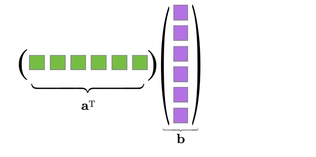
Figure 2.5: Animation of Inner Product between two vectors

Example 2.5 (Vector Inner Product) Let \[\x=\left(\begin{matrix} -1 \\2\\4\\0 \end{matrix}\right) \quad \y=\left(\begin{matrix} 3 \\5\\1\\7 \end{matrix}\right) \quad \v=\left(\begin{matrix} -3 \\-2\\5\\3\\-2 \end{matrix}\right) \quad \u= \left(\begin{matrix} 2\\-1\\3\\-3\\-2 \end{matrix}\right)\]

If possible, compute the following inner products:

1. \(\x^T\y\) \[\begin{eqnarray} \x^T\y &=&\left(\begin{matrix} -1 &2&4&0 \end{matrix}\right) \left(\begin{matrix} 3 \\5\\1\\7 \end{matrix}\right) \cr &=& (-1)(3)+(2)(5)+(4)(1)+(0)(7) \cr &=& -3+10+4=\framebox{11} \end{eqnarray}\]
2. \(\x^T\v\) This is not possible because \(\x\) and \(\v\) do not have the same number of elements
3. \(\v^T\u\) \[\begin{eqnarray} \v^T\u &=& \left(\begin{matrix} -3 &-2&5&3&-2 \end{matrix}\right) \left(\begin{matrix} 2\\-1\\3\\-3\\-2 \end{matrix}\right) \cr &=& (-3)(2)+(-2)(-1)+(5)(3)+(3)(-3)+(-2)(-2) \cr &=& -6+2+15-9+4 = \framebox{6} \end{eqnarray}\]

Exercise 2.2 (Vector Inner Product) Let \[\bo{v}=\left(\begin{matrix} 1 \\2\\3\\4\\5 \end{matrix}\right) \quad \e=\left(\begin{matrix} 1 \\1\\1\\1\\1 \end{matrix}\right) \quad \bo{p}=\left(\begin{matrix} 0.5 \\0.1\\0.2\\0\\0.2 \end{matrix}\right) \quad \u= \left(\begin{matrix} 10\\4\\3\\2\\1 \end{matrix}\right) \quad \bo{s} = \left(\begin{matrix} 2\\2\\-3 \end{matrix}\right)\]

If possible, compute the following inner products:

1. \(\bo{v}^T\e\)
2. \(\bo{e}^T\bo{v}\)
3. \(\bo{v}^T\bo{s}\)
4. \(\bo{p}^T\u\)
5. \(\bo{v}^T\bo{v}\)

It should be clear from the definition and from the previous exercise, that for all vectors \(\x\) and \(\y\), \[\x^T\y = \y^T\x.\] Also, if we take the inner product of a vector with itself, the result is the sum of squared elements in that vector: \[\x^T\x = \sum_{i=1}^n x_i^2 = x_1^2 + x_2^2+ \dots + x_n^2.\]

Now that we are comfortable multiplying a row vector (\(\x^T\) in the definition) and a column vector (\(\y\) in the definition), we can define multiplication for matrices in general.

2.4.2 Matrix Product

Matrix multiplication is nothing more than a collection of inner products done simultaneously in one operation. We must be careful when multiplying matrices because, as with vectors, the operation is not always possible. Unlike the vector inner product, the order in which you multiply matrices makes a big difference!

Definition 2.4 (Matrix Multiplication) Let \(\mathbf{A}_{m\times n}\) and \(\mathbf{B}_{k\times p}\) be matrices. The matrix product \(\mathbf{A}\mathbf{B}\) is possible if and only if \(n=k\); that is, when the number of columns in \(\mathbf{A}\) is the same as the number of rows in \(\mathbf{B}\). If this condition holds, then the dimension of the product, \(\mathbf{A}\mathbf{B}\) is \(m\times p\) and the (ij)-entry of the product \(\mathbf{A}\mathbf{B}\) is the inner product of the \(i^{th}\) row of \(\mathbf{A}\) and the \(j^{th}\) column of \(\mathbf{B}\):

\[(\mathbf{A}\mathbf{B})_{ij} = \mathbf{A}_{i\star}\mathbf{B}_{\star j}\]

This definition may be easier to dissect using an example:

Example 2.6 (Steps to Compute a Matrix Product) Let \[\mathbf{A}=\left(\begin{matrix} 2 & 3 \\ -1 & 4 \\ 5 & 1 \end{matrix}\right) \quad \mbox{and} \quad \mathbf{B}=\left(\begin{matrix} 0 & -2 \\ 2 & -3 \end{matrix}\right)\]

When we first get started with matrix multiplication, we often follow a few simple steps:

1. Write down the matrices and their dimensions. Make sure the “inside” dimensions match - those corresponding to the columns of the first matrix and the rows of the second matrix: \[\underset{(3\times \red{2})}{\mathbf{A}} \underset{(\red{2} \times 2)}{\mathbf{B}}\] If these dimensions match, then we can multiply the matrices. If they don’t, we stop right there - multiplication is not possible.
2. Now, look at the “outer” dimensions - this will tell you the size of the resulting matrix. \[\underset{(\blue{3}\times 2)}{\mathbf{A}} \underset{(2\times \blue{2})}{\mathbf{B}}\] So the product \(\mathbf{A}\mathbf{B}\) is a \(3\times 2\) matrix.
3. Finally, we compute the product of the matrices by multiplying each row of \(\mathbf{A}\) by each column of \(\mathbf{B}\) using inner products. The element in the first row and first column of the product (written \((\mathbf{A}\mathbf{B})_{11}\)) will be the inner product of the first row of \(\mathbf{A}\) and the first column of \(\mathbf{B}\). Then, \((\mathbf{A}\mathbf{B})_{12}\) will be the inner product of the first row of \(\mathbf{A}\) and the second column of \(\mathbf{B}\), etc.

\[\begin{eqnarray} \mathbf{A}\mathbf{B} &=&\left(\begin{matrix} (2)(0)+(3)(2) & (2)(-2)+(3)(-3)\\ (-1)(0)+(4)(2) & (-1)(-2)+(4)(-3)\\ (5)(0)+(1)(2) & (5)(-2)+(1)(-3) \end{matrix}\right) \cr &=& \left(\begin{matrix} 6&-13\\8 & -10\\2&-13\end{matrix}\right) \end{eqnarray}\]

Matrix multiplication is incredibly important for data analysis. You may not see why all these multiplications and additions are so useful at this point, but we will visit some basic applications shortly. For now, let’s practice so that we are prepared for the applications!

Exercise 2.3 (Matrix Multiplication) Suppose we have \[\mathbf{A}_{4\times 6} \quad \mathbf{B}_{5\times 5} \quad \M_{5\times 4} \quad \bP_{6\times 5}\] Circle the matrix products that are possible to compute and write the dimension of the result. \[\mathbf{A}\M \qquad \M\mathbf{A} \qquad \mathbf{B}\M \qquad \M\mathbf{B} \qquad \bP\mathbf{A} \qquad \bP\M \qquad \mathbf{A}\bP \qquad \mathbf{A}^T\bP \qquad \M^T\mathbf{B}\] Let \[\begin{equation} \mathbf{A}=\left(\begin{matrix} 1&1&0&1\\0&1&1&1\\1&0&1&0\end{matrix}\right) \quad \M = \left(\begin{matrix} -2&1&-1&2&-2\\1&-2&0&-1&2\\2&1&-3&-2&3 \\ 1&3&2&-1&2\end{matrix}\right) \end{equation}\]

\[\begin{equation} \C=\left(\begin{matrix} -1&0&1&0\\1&-1&0&0\\0&0&1&-1 \end{matrix}\right) \end{equation}\]

Determine the following matrix products, if possible:

1. \(\mathbf{A}\C\)

2. \(\mathbf{A}\M\)

3. \(\mathbf{A}^T\C\)

One very important thing to keep in mind is this:

matrix multiplication is NOT commutative!

As we see from the previous exercises, it’s quite common to be able to compute a product \(\mathbf{A}\mathbf{B}\) where the reverse product, \(\mathbf{B}\mathbf{A}\) is not even possible to compute. Even if both products are possible it is almost never the case that \(\mathbf{A}\mathbf{B}\) equals \(\mathbf{B}\mathbf{A}\).

2.4.3 Matrix-Vector Product

A matrix-vector product works exactly the same way as matrix multiplication; after all, a vector \(\x\) is nothing but an \(n\times 1\) matrix. In order to multiply a matrix by a vector, again we must match the dimensions to make sure they line up correctly. For example, if we have an \(m\times n\) matrix \(\mathbf{A}\), we can multiply by a \(1\times m\) row vector \(\v^T\) on the left: \[\v^T\mathbf{A} \quad \mbox{works because } \underset{ (1\times \red{m})}{\v^T} \underset{(\red{m}\times n)}{\mathbf{A}}\] \[\Longrightarrow \mbox{The result will be a } 1 \times n \mbox{ row vector.}\] or we can multiply by an \(n\times 1\) column vector \(\x\) on the right:

\[\mathbf{A}\x \quad \mbox{works because } \underset{(m\times \red{n})}{\mathbf{A}}\underset{(\red{n}\times 1)}{\x} \] \[\Longrightarrow \mbox{The result will be a } m\times 1 \mbox{ column vector.}\]

Matrix-vector multiplication works the same way as matrix multiplication: we simply multiply rows by columns until we’ve completed the answer. In the case of \(\v^T\mathbf{A}\), we’d multiply the row \(\v\) by each of the \(n\) columns of \(\mathbf{A}\), carving out our solution, one entry at a time :

\[\v^T\mathbf{A} = \left(\begin{matrix} \v^T\mathbf{A}_{*1} & \v^T\acol{2} & \dots & \v^T\acol{n} \end{matrix}\right).\]

In the case of \(\mathbf{A}\x\), we’d multiply each of the \(m\) rows of \(\mathbf{A}\) by the column \(\x\):

\[\mathbf{A}\x = \left(\begin{matrix} \arow{1}\x \\ \arow{2}\x \\ \vdots \\ \arow{m}\x \end{matrix}\right).\]

Let’s see an example of this:

Example 2.7 (Matrix-Vector Products) Let \[\mathbf{A}=\left(\begin{matrix} 2 & 3 \\ -1 & 4 \\ 5 & 1 \end{matrix}\right) \quad \v=\left(\begin{matrix} 3\\2 \end{matrix}\right) \quad \bo{q}=\left(\begin{matrix} 2\\-1\\3\end{matrix}\right)\]

Determine whether the following matrix-vector products are possible. When possible, compute the product.

1. \(\mathbf{A}\bo{q}\) \[\mbox{Not Possible: Inner dimensions do not match} \quad \underset{(3\times \red{2})}{\mathbf{A}}\underset{(\red{3}\times 1)}{\bo{q}}\]

2. \(\mathbf{A}\v\) \[ \left(\begin{matrix} 2 & 3 \\ -1 & 4 \\ 5 & 1 \end{matrix}\right) \left(\begin{matrix} 3\\2 \end{matrix}\right) = \left(\begin{matrix} 2(3)+3(2) \\ -1(3)+4(2)\\5(3)+1(2) \end{matrix}\right) = \left(\begin{matrix} 12\\5\\17\end{matrix}\right) \]

3. \(\bo{q}^T\mathbf{A}\)

   Rather than write out the entire calculation, the blue text highlights one of the two inner products required:

   \[ \left(\begin{matrix} \blue{2} & \blue{-1} & \blue{3}\end{matrix}\right) \left(\begin{matrix} \blue{2} & 3 \\ \blue{-1} & 4 \\ \blue{5} & 1 \end{matrix}\right) = \left(\begin{matrix} \blue{20} & 5 \end{matrix}\right) \]

4. \(\v^T\mathbf{A}\) \[\mbox{Not Possible: Inner dimensions do not match} \quad \underset{(1\times \red{2})}{\v^T}\underset{(\red{3}\times 2)}{\mathbf{A}}\]

Exercise 2.4 (Matrix-Vector Products) Let \[ \mathbf{A}=\left(\begin{matrix} 1&1&0&1\\0&1&1&1\\1&0&1&0\end{matrix}\right) \quad \mathbf{B}=\left(\begin{matrix} 0 & -2 \\ 1 & -3 \end{matrix}\right) \] \[ \x=\left(\begin{matrix} 2\\1\\3 \end{matrix}\right) \quad \y = \left(\begin{matrix} 1\\1 \end{matrix}\right) \quad \z = \left(\begin{matrix} 3\\1\\2\\3 \end{matrix}\right)\] Determine whether the following matrix-vector products are possible. When possible, compute the product.

1. \(\mathbf{A}\z\)

2. \(\z^T\mathbf{A}\)

3. \(\y^T\mathbf{B}\)

4. \(\mathbf{B}\y\)

5. \(\x^T\mathbf{A}\)

Linear Combination view of Matrix Products

All matrix products can be viewed as linear combinations or a collection of linear combinations. This vantage point is extremely crucial to our understanding of data science techniques that are based on matrix-factorization. Let’s start with matrix-vector product and see how we can depict it as a linear combination of the columns of the matrix.

Definition 2.5 (Matrix-Vector Product as a Linear Combination) Let \(\mathbf{A}\) be an \(m\times n\) matrix partitioned into columns, \[\mathbf{A} = [\mathbf{A}_1 | \mathbf{A}_2 | \dots | \mathbf{A}_n]\] and let \(\x\) be a vector in \(\Re^n\). Then, \[\mathbf{A}\x = x_1\mathbf{A}_1 + x_2\mathbf{A}_2 + \dots + x_n\mathbf{A}_n\]

We use the animation in Figure 2.6 to illustrate Definition 2.5.

Figure 2.6: Illustration of Definition 2.5

Definition 2.5 extends to any matrix product. If \(\mathbf{A}\mathbf{B}=\mathbf{C}\) then the columns of \(\mathbf{C}\) can be viewed as linear combinations of the columns of \(\mathbf{A}\) and, likewise, the rows of \(\C\) can be viewed as linear combinations of the rows of \(\mathbf{B}\). We leave the latter fact for the reader to explore independently (see end-of-chapter exercise 5), and animate the former in Figure 2.7.

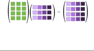
Figure 2.7: Illustration of Definition 2.5

2.4.3.1 Multiplication by a Diagonal Matrix

As we will see in the next example, multiplication by a diagonal matrix causes a very specific effect on a matrix.

Example 2.8 (Multiplication by a Diagonal Matrix) Compute the following matrix product and comment on what you find in the results: \[\D=\left(\begin{matrix} 2&0&0\\0&3&0\\0&0&-2 \end{matrix}\right) \mathbf{A}= \left(\begin{matrix} 1&2&3\\1&1&2\\2&1&3 \end{matrix}\right)\] \[\D\mathbf{A}=\left(\begin{matrix} 2&4&6\\3&3&6\\-4&-2&-6 \end{matrix}\right)\] In doing this multiplication, we see that the effect of multiplying the matrix \(\mathbf{A}\) by a diagonal matrix on the left is that the rows of the matrix \(\mathbf{A}\) are simply scaled by the entries in the diagonal matrix. You should work this computation out by hand to convince yourself that this effect will happen every time. Diagonal scaling can be important, and from now on when you see a matrix product like \(\D\mathbf{A}\) where \(\D\) is diagonal, you should automatically put together that the result is just a row-scaled version of \(\mathbf{A}\).

Exercise 2.5 (Multiplication by a Diagonal Matrix) What happens if we were to compute the product from Example 2.8 in the reversed order, with the diagonal matrix on the right: \(\mathbf{A}\D?\)
Would we expect the same result? Is multiplication by a diagonal matrix commutative? Work out the calculation and comment on what you’ve found.

2.5 Vector Outer Products

Inner products involved multiplying a row vector by a column vector on the right (think \(\x^T\y\)). Outer products occur when we multiply a column vector with a row vector on the right (think \(\x\y^T\)). Let’s first consider the dimensions of the outcome:

\[\underset{(m\times \red{1})}{\x} \underset{(\red{1} \times n)}{\y^T} = \bo{M}_{m\times n}\]

So the result is a matrix! We’ll want to treat this product in the same way we treat any matrix product, by multiplying row \(\times\) column until we’ve run out of rows and columns. Let’s take a look at an example:

Example 2.9 (Vector Outer Product) Let \(\x = \left(\begin{matrix} 3\\4\\-2 \end{matrix}\right)\) and \(\y=\left(\begin{matrix} 1\\5\\3 \end{matrix}\right)\). Then, \[\x\y^T = \left(\begin{matrix} \red{3}\\4\\-2 \end{matrix}\right) \left(\begin{matrix} \red{1}&5&3 \end{matrix}\right) = \left(\begin{matrix} \red{3}&15&9\\4&20&12\\-2&-10&-3\end{matrix}\right)\] As you can see by performing this calculation, a vector outer product will always produce a matrix whose rows are multiples of each other!

Example 2.10 (Centering Data with an Outer Product) As we’ve seen in previous examples, many statistical formulas involve the centered data, that is, data from which the mean has been subtracted so that the new mean is zero. Suppose we have a matrix of data containing observations of individuals’ heights (h) in inches, weights (w), in pounds and wrist sizes (s), in inches:

\[\begin{equation}\A=\begin{array}{cc} & \begin{array}{ccc} h & w & s \end{array} \\ \begin{array}{c} person_1 \\ person_2 \\ person_3 \\ person_4 \\ person_5 \end{array} & \left(\begin{array}{ccc}60 & 102 & 5.5 \cr 72 & 170 & 7.5 \cr 66 & 110 & 6.0\cr 69 & 128 & 6.5\cr 63 & 130 & 7.0\cr \end{array} \right)\end{array}\end{equation}\]

The average values for height, weight, and wrist size are as follows: \[\begin{eqnarray} \bar{h}&=&66\\ \bar{w}&=&128\\ \bar{s}&=&6.5 \end{eqnarray}\]

To center all of the variables in this data set simultaneously, we could compute an outer product using a vector containing the means and a vector of all ones:

\[\pm 60 & 102 & 5.5 \cr 72 & 170 & 7.5 \cr 66 & 110 & 6.0\cr 69 & 128 & 6.5\cr 63 & 130 & 7.0\cr \mp - \pm 1\\1\\1\\1\\1 \mp \pm 66 & 128 & 6.5 \mp\] \[= \pm 60 & 102 & 5.5 \cr 72 & 170 & 7.5 \cr 66 & 110 & 6.0\cr 69 & 128 & 6.5\cr 63 & 130 & 7.0\cr \mp - \pm 66 & 128 & 6.5 \\66 & 128 & 6.5 \\66 & 128 & 6.5 \\66 & 128 & 6.5 \\66 & 128 & 6.5 \mp\]

\[= \pm -6.0000 & -26.0000 & -1.0000\\ 6.0000 & 42.0000 & 1.0000\\ 0 & -18.0000 & -0.5000\\ 3.0000 & 0 & 0\\ -3.0000 & 2.0000 & 0.5000 \mp\]

2.6 The Identity and the Matrix Inverse

The identity matrix, introduced in Section 1.6, is to matrices as the number `1’ is to scalars. It is the multiplicative identity. For any matrix (or vector) \(\mathbf{A}\), multiplying \(\mathbf{A}\) by the identity matrix on either side does not change \(\mathbf{A}\): \[\begin{align*} \mathbf{A}\I&=\mathbf{A} \\ \I\mathbf{A} &= \mathbf{A} \end{align*}\]

This fact is easy to verify in light of Example 2.8. Since the identity is simply a diagonal matrix with ones on the diagonal, when we multiply it by any matrix it merely scales each row or column of that matrix by 1. The size of the identity matrix is generally implied in context. If \(\mathbf{A}\) is \(m\times n\) then writing \(\mathbf{A}\I\) implies that \(\I\) is \(n \times n\), where as writing \(\I\mathbf{A}\) implies \(\I\) is \(m\times m\).

For certain square matrices \(\mathbf{A}\), an inverse matrix, written \(\mathbf{A}^{-1}\), exists such that \[\mathbf{A}\mathbf{A}^{-1} = \I\] \[\mathbf{A}^{-1}\mathbf{A} = \I\] It is very important to understand that not all matrices have inverses. There are 2 very important conditions that must be satisfied:

We have not yet discussed the notion of matrix rank, so the present discussion is aimed only at defining the concept of a matrix inverse rather than defining when it exists or how it is determined. For now, we want to see the analogy of the matrix inverse to our previous understanding of scalar algebra. Recall that the inverse of a non-zero scalar number is its reciprocal: \[a^{-1} = \frac{1}{a}\] Multiplying a scalar by its inverse yields the multiplicative identity, 1: \[(a)(a^{-1}) = (a)(\frac{1}{a}) = 1\] All scalars have an inverse with the exception of 0. For matrices, the idea of an inverse is quite the same - multiply a matrix on the left or right by its inverse to get the multiplicative identity, \(\I\). However, as previously stated, the matrix inverse only exists for a small subset of matrices, those that are square and full rank. Such matrices are equivalently called invertible or non-singular.

Example 2.11 (Don’t Cancel That!!) We must be careful in linear algebra to remember the basics and not confuse our equations with scalar equations. When we see an equation like \[\mathbf{A}\x=\lambda\x\] We CANNOT cancel terms from both sides. Mathematically, this operation amounts to multiplying both sides by an inverse. When the term we are canceling is a non-zero scalar, then we can proceed as usual. However, we must be careful not to assume that a matrix/vector quantity has an inverse. For example, the following operation is nonsense: \[\require{cancel}\] \[\mathbf{A}\cancel{\mathbf{x}}=\lambda \cancel{\mathbf{x}}\] Note that, while this equation made sense to begin with, after erroneously canceling terms, it no longer makes sense as it equates a matrix, \(\mathbf{A}\), with a scalar, \(\lambda\).

2.7 Exercises

1. On a coordinate plane, draw the vectors \(\a = \left(\begin{matrix} 1\\2\end{matrix}\right)\) and \(\b=\left(\begin{matrix} 0\\1\end{matrix}\right)\) and then draw \(\bo{c}=\a+\b\). Make dotted lines which illustrate how the point/vector \(\bo{c}\) can be reached by connecting the vectors a and b “tail-to-head.”
2. Use the following vectors to answer the questions: \[ \v=\left(\begin{matrix} 6\\-1\end{matrix}\right) \quad \bo{u}=\left(\begin{matrix} -2\\1\end{matrix}\right) \quad \x=\left(\begin{matrix} 4\\2\\1\end{matrix}\right) \quad \y=\left(\begin{matrix}-1\\-2\\-3\end{matrix}\right) \quad \e=\left(\begin{matrix} 1\\1\\1\end{matrix}\right) \]
   1. Compute the following linear combinations, if possible:
      1. \(2\u+3\v=\)
      2. \(\x-2\y+\e=\)
      3. \(-2\u-\v+\e=\)
      4. \(\u+\e=\)
   2. Compute the following inner products, if possible:
      1. \(\u^T\v=\)
      2. \(\x^T\x=\)
      3. \(\e^T\y=\)
      4. \(\x^T\u=\)
      5. \(\x^T\e=\)
      6. \(\y^T\e=\)
      7. \(\v^T\x=\)
      8. \(\e^T\v=\)
         
   3. What happens when you take the inner product of a vector with \(\e\)?
      
   4. What happens when you take the inner product of a vector with itself (as in \(\x^T\x\))?
      
3. Use the following matrices to answer the questions: \[\mathbf{A}=\left(\begin{matrix} 1&3&8\\3&0&-2\\8&-2&-3 \end{matrix}\right) \quad \bo{M}=\left(\begin{matrix} 1&8&-2&5\\2&8&1&7 \end{matrix}\right) \quad \D = \left(\begin{matrix} 1&0&0\\0&5&0\\0&0&3\end{matrix}\right) \] \[ \bo{H}=\left(\begin{matrix} 2&-1\\1&3 \end{matrix}\right) \quad \bo{W}=\left(\begin{matrix} 1&1&1&1\\2&2&2&2\\3&3&3&3\end{matrix}\right) \]
   1. Circle the matrix products that are possible and specify their resulting dimensions:
      1. \(\mathbf{A}\M\)
      2. \(\mathbf{A}\bo{W}\)
      3. \(\bo{W}\D\)
      4. \(\bo{W}^T\D\)
      5. \(\bo{H}\M\)
      6. \(\bo{M}\bo{H}\)
      7. \(\bo{M}^T\bo{H}^T\)
      8. \(\D\bo{W}\)
         

   2. Compute the following matrix products:

      \[\bo{H}\M\quad \mbox{and} \quad \mathbf{A}\D\]
   3. From the previous computation, \(\mathbf{A}\D\), do you notice anything interesting about multiplying a matrix by a diagonal matrix on the right? Can you generalize what happens in words? (Hint: see Example 2.8 and Exercise 2.5.
      
4. Is matrix multiplication commutative?
5. Different Views of Matrix Multiplication: Consider the matrix product \(\mathbf{A}\mathbf{B}\) where \[\mathbf{A} = \left(\begin{matrix} 1 & 2\\3&4 \end{matrix}\right) \quad \mathbf{B} = \left(\begin{matrix} 2&5\\1&3\end{matrix}\right)\] Let \(\C=\mathbf{A}\mathbf{B}\).
   1. Compute the matrix product \(\C\).
   2. Compute the matrix-vector product \(\mathbf{A}\mathbf{B}_{\star 1}\) and show that this is the first column of \(\C\). (Likewise, \(\mathbf{A}\mathbf{B}_{\star 2}\) is the second column of \(\C\).) (Matrix multiplication can be viewed as a collection of matrix-vector products.)
   3. Compute the two outer products using columns of \(\mathbf{A}\) and rows of \(\mathbf{B}\) and show that \[\acol{1}\brow{1} + \acol{2}\brow{2} = \C\] (Matrix multiplication can be viewed as the sum of outer products.)
   4. Since \(\mathbf{A}\mathbf{B}_{\star 1}\) is the first column of \(\C\), show how \(\C_{\star 1}\) can be written as a linear combination of columns of \(\mathbf{A}\). (Matrix multiplication can be viewed as a collection of linear combinations of columns of the first matrix.)
   5. Finally, note that \(\arow{1}\mathbf{B}\) will give the first row of \(\C\). (This amounts to a linear combination of rows - can you see that?)
6. For the matrix \(\bo{H} = \X(\X^T\cov^{-1}\X)^{-1}\X^T\cov^{-1}\), use the properties of matrix arithmetic to show that
   1. \(\bo{H}^2 = \bo{H}\)
   2. \(\bo{H}(\I-\bo{H}) = \bo{0}\)
7. Suppose we measure the heights of 10 people, \(person_1, person_2, \dots, person_{10}\).
   1. If we create a matrix \(\S\) where \[S_{ij} = height(person_i) - height(person_j)\] is the matrix \(\S\) symmetric? What is the trace(\(\S\))?
   2. If instead we create a matrix \(\bo{G}\) where \[G_{ij} = [height(person_i) - height(person_j)]^2\] is the matrix \(\bo{G}\) symmetric? What is the trace(\(\bo{G}\))?

List of Key Terms

• addition
• subtraction
• equal matrices
• scalar multiplication
• inner product
• matrix product
• linear combination
• outer product
• multiplicative identity
• matrix inverse