Chapter 11 Applications of Least Squares
11.1 Simple Linear Regression
11.1.1 Cars Data
The `cars’ dataset is included in the datasets package. This dataset contains observations of speed and stopping distance for 50 cars. We can take a look at the summary statistics by using the summary function.
summary(cars)## speed dist
## Min. : 4.0 Min. : 2.00
## 1st Qu.:12.0 1st Qu.: 26.00
## Median :15.0 Median : 36.00
## Mean :15.4 Mean : 42.98
## 3rd Qu.:19.0 3rd Qu.: 56.00
## Max. :25.0 Max. :120.00We can plot these two variables as follows:
plot(cars)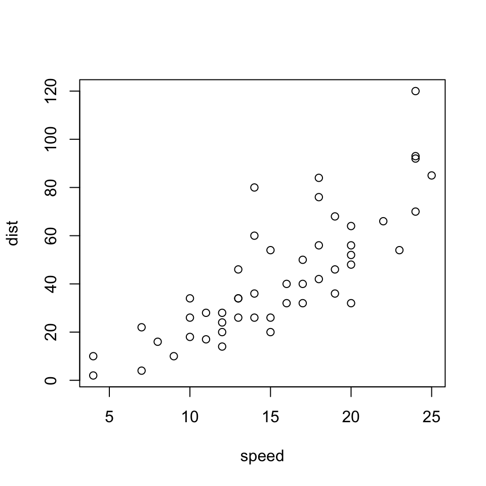
11.1.2 Setting up the Normal Equations
Let’s set up a system of equations \[\mathbf{X}\boldsymbol\beta=\mathbf{y}\] to create the model \[stopping\_distance=\beta_0+\beta_1speed.\]
To do this, we need a design matrix \(\mathbf{X}\) containing a column of ones for the intercept term and a column containing the speed variable. We also need a vector \(\mathbf{y}\) containing the corresponding stopping distances.
The model.matrix() function
The model.matrix() function will create the design or modeling matrix \(\mathbf{X}\) for us. This function takes a formula and data matrix as input and exports the matrix that we represent as \(\mathbf{X}\) in the normal equations. For datasets with categorical (factor) inputs, this function would also create dummy variables for each level, leaving out a reference level by default. You can override the default to leave out a reference level (when you override this default, you perform one-hot-encoding on said categorical variable) by including the following option as a third input to the function, where df is the name of your data frame:
contrasts.arg = lapply(df[,sapply(df,is.factor) ], contrasts, contrasts=FALSE
For an exact example, see the commented out code in the chunk below. There are no factors in the cars data, so the code may not even run, but I wanted to provide the line of code necessary for this task, as it is one that we use quite frequently for clustering, PCA, or machine learning!
# Create matrix X and label the columns
X=model.matrix(dist~speed, data=cars)
# Create vector y and label the column
y=cars$dist


# CODE TO PERFORM ONE-HOT ENCODING (NO REFERENCE LEVEL FOR CATEGORICAL DUMMIES)
# X=model.matrix(dist~speed, data=cars, contrasts.arg = lapply(cars[,sapply(cars,is.factor) ], contrasts, contrasts=FALSE)
Let’s print the first 10 rows of each to see what we did:
# Show first 10 rows, all columns. To show only observations 2,4, and 7, for
# example, the code would be X[c(2,4,7), ]
X[1:10, ]
## (Intercept) speed
## 1 1 4
## 2 1 4
## 3 1 7
## 4 1 7
## 5 1 8
## 6 1 9
## 7 1 10
## 8 1 10
## 9 1 10
## 10 1 11y[1:10]## [1] 2 10 4 22 16 10 18 26 34 1711.1.3 Solving for Parameter Estimates and Statistics
Now lets find our parameter estimates by solving the normal equations,
\[\mathbf{X}^T\mathbf{X}\boldsymbol\beta = \mathbf{X}^T\mathbf{y}\]
using the built in solve function. To solve the system \(\mathbf{A}\mathbf{x}=\mathbf{b}\) we’d use solve(A,b).
(beta=solve(t(X) %*% X ,t(X)%*%y))## [,1]
## (Intercept) -17.579095
## speed 3.932409At the same time we can compute the residuals, \[\mathbf{r}=\mathbf{y}-\mathbf{\hat{y}}\] the total sum of squares (SST), \[\sum_{i=1}^n (y-\bar{y})^2=(\mathbf{y}-\mathbf{\bar{y}})^T(\mathbf{y}-\mathbf{\bar{y}})=\|\mathbf{y}-\mathbf{\bar{y}}\|^2\] the regression sum of squares (SSR or SSM) \[\sum_{i=1}^n (\hat{y}-\bar{y})^2=(\mathbf{\hat{y}}-\mathbf{\bar{y}})^T(\mathbf{\hat{y}}-\mathbf{\bar{y}})=\|\mathbf{\hat{y}}-\mathbf{\bar{y}}\|^2\] the residual sum of squares (SSE) \[\sum_{i=1}^n r_i =\mathbf{r}^T\mathbf{r}=\|\mathbf{r}\|^2\] and the unbiased estimator of the variance of the residuals, using the model degrees of freedom which is \(n-2=48\): \[\widehat{\sigma_{\varepsilon}}^2 =\frac{SSE}{d.f.} = \frac{\|\mathbf{r}\|^2}{48}\]
Then \(R^2\): \[R^2 = \frac{SSR}{SST}\]
We can also compute the standard error of \(\widehat{\boldsymbol\beta}\) since
\[\begin{eqnarray*} \widehat{\boldsymbol\beta} &=& (\mathbf{X}^T\mathbf{X})^{-1}\mathbf{X}^T\mathbf{y}\\ var(\widehat{\boldsymbol\beta})&=&var((\mathbf{X}^T\mathbf{X})^{-1}\mathbf{X}^T\mathbf{y})\\ &=&(\mathbf{X}^T\mathbf{X})^{-1}\mathbf{X}^T var(\mathbf{y}) \mathbf{X}(\mathbf{X}^T\mathbf{X})^{-1} \\ &=&(\mathbf{X}^T\mathbf{X})^{-1}\mathbf{X}^T (\widehat{\sigma_{\varepsilon}}^2) \mathbf{X}(\mathbf{X}^T\mathbf{X})^{-1} \\ &=& \widehat{\sigma_{\varepsilon}}^2 (\mathbf{X}^T\mathbf{X})^{-1}\mathbf{X}^T\mathbf{X}(\mathbf{X}^T\mathbf{X})^{-1} \\ &=& \widehat{\sigma_{\varepsilon}}^2(\mathbf{X}^T\mathbf{X})^{-1} \end{eqnarray*}\]
The variances of each \(\widehat\beta\) are given by the diagonal elements of their covariance matrix (see Definition 6.3), and the standard errors of each \(\widehat\beta\) are thus obtained by taking the square roots of these diagonal elements: \[s.e.(\widehat{\beta_i})=\sqrt{\widehat{\sigma_{\varepsilon}}[(\mathbf{X}^T\mathbf{X})^{-1}]_{ii}}\]
meany=mean(y)
XXinv=solve(t(X)%*%X)
yhat=X%*%XXinv%*%t(X)%*%y
resid=y-yhat
SStotal=norm(y-meany,type="2")^2
### OR  SStotal=t(y-meany)%*%(y-meany)
SSreg=norm(yhat-meany,type="2")^2
### OR  SSreg=t(yhat-meany)%*%(yhat-meany)
SSresid=norm(resid,type="2")^2
### OR SSresid=t(resid)%*%resid
Rsquared=SSreg/SStotal
StdErrorResiduals=norm(resid/sqrt(48), type="2") #=sqrt(SSresid/48)
CovBeta=SSresid*XXinv/48
StdErrorIntercept = sqrt(CovBeta[1,1])
StdErrorSlope = sqrt(CovBeta[2,2])
## [1] "Rsquared: 0.651079380758252"## [1] "SSresid: 11353.5210510949"## [1] "SSmodel: 21185.4589489052"## [1] "StdErrorResiduals: 15.3795867488199"## [1] "StdErrorIntercept: 6.75844016937923"## [1] "StdErrorIntercept: 0.415512776657122"Let’s plot our regression line over the original data:
plot(cars)
abline(beta[1],beta[2],col='blue')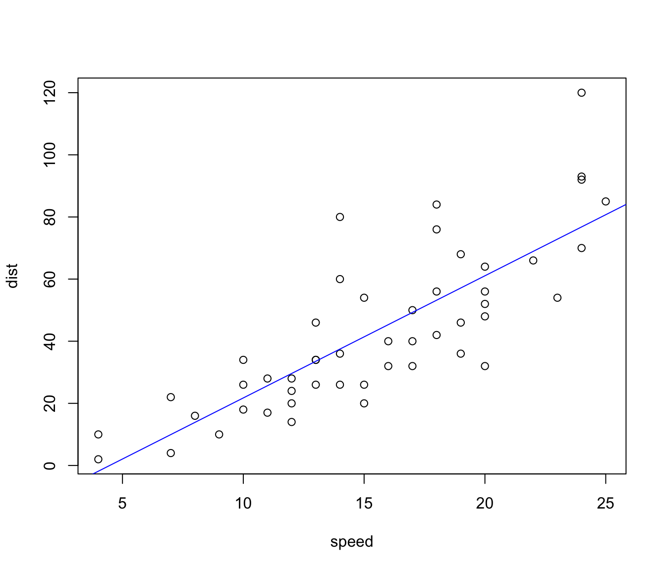
11.1.4 OLS in R via lm()
Finally, let’s compare our results to the built in linear model solver, lm():
fit = lm(dist ~ speed, data=cars)
summary(fit)
##
## Call:
## lm(formula = dist ~ speed, data = cars)
##
## Residuals:
## Min 1Q Median 3Q Max
## -29.069 -9.525 -2.272 9.215 43.201
##
## Coefficients:
## Estimate Std. Error t value Pr(>|t|)
## (Intercept) -17.5791 6.7584 -2.601 0.0123 *
## speed 3.9324 0.4155 9.464 1.49e-12 ***
## ---
## Signif. codes: 0 '***' 0.001 '**' 0.01 '*' 0.05 '.' 0.1 ' ' 1
##
## Residual standard error: 15.38 on 48 degrees of freedom
## Multiple R-squared: 0.6511, Adjusted R-squared: 0.6438
## F-statistic: 89.57 on 1 and 48 DF, p-value: 1.49e-12anova(fit)## Analysis of Variance Table
##
## Response: dist
## Df Sum Sq Mean Sq F value Pr(>F)
## speed 1 21186 21185.5 89.567 1.49e-12 ***
## Residuals 48 11354 236.5
## ---
## Signif. codes: 0 '***' 0.001 '**' 0.01 '*' 0.05 '.' 0.1 ' ' 1