Chapter 21 Algorithms for Data Clustering
There have been countless algorithms proposed for data clustering. While a complete survey and discussion of clustering algorithms would be nearly impossible, this chapter provides an introduction to some of the most popular algorithms to date. For the purposes of organization, the algorithms are divided into 3 groups: Hierarchical, Iterative Partitional, and Density-based.
21.1 Hierarchical Algorithms
As discussed in Chapter 20, data clustering became popular in the biological fields of phylogeny and taxonomy. Even prior to the advancement of numerical taxonomy, it was common for scientists in this field to communicate relationships by way of a dendrogram or tree diagram as illustrated in Figure 21.1 [51]. Dendrograms provide a nested hierarchy of similarity that allow the researcher to see different levels of clustering that may exist in data, particularly in phylogenic data. Agglomerative hierarchical clustering has its roots in this domain.
21.1.1 Agglomerative Hierarchical Clustering
The idea behind agglomerative heirarchical clustering is to link similar objects or similar clusters of objects together in a hierarchy where the highest levels of similarity is represented by the lowest level connections. These methods are called agglomerative because they begin with each data point in a separate cluster and at each step they merge clusters together according to some decision rule until eventually all of the points end up in a single cluster. For example, in Figure 21.1, objects 1 and 2 exhibit the highest level of similarity as indicated by the height of the branch that connects them. Also illustrated in the dendrogram is the fact that the blue cluster and green cluster are more similar to each other than they are to the red cluster. One of the advantages to these hierarchical structures is that branches can be cut to achieve any number of clusters desired by the user. For example, in Figure 21.1 if only the highest branch of the dendrogram is cut, the result is two clusters: {{1,2,3},{4,5,6,7,8,9}}. When the next highest branch is cut, we are left with 3 clusters: {{1,2,3},{4,5,6},{7,8,9}}.
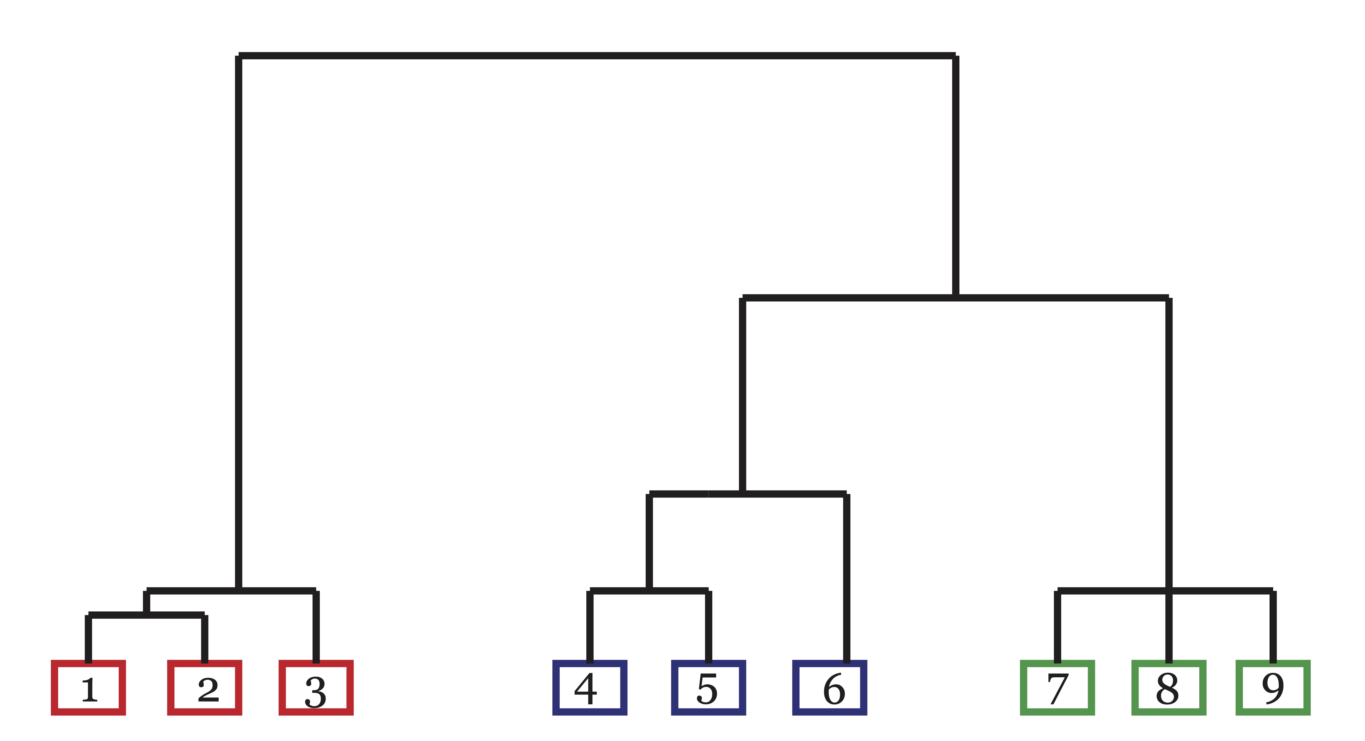
Figure 21.1: A Dendrogram exhibiting linkage/similarity between 9 objects in 3 clusters.
There are a number of different systems for determining linkage in hierarchical clustering dendrograms. For a complete discussion, we suggests the classic books by Anderberg [43] or Jain and Dubes [42]. The basic scheme for hierarchical clustering algorithms is outlined in the algorithm below.
- Input: n objects to be clustered.
- Begin by assigning each object to its own cluster.
- Compute the pairwise similarities between each cluster.
- Find the most similar pair of clusters and merge them into a single cluster. There is now one less cluster.
- Compute pairwise similarities between the new cluster and each of the old clusters.
- Repeat steps 3-4 until all objects belong to a single cluster of size n.
- Output: Dendrogram depicting each merge step.
What differentiates the numerous hierarchical clustering algorithms is the choice of similarity metric used and the way the chosen similarity metric is used to compare clusters in step 4. For example, suppose Euclidean distance is chosen to compute the similarity (or dissimilarity) between objects in step 2. In step 4, the same notion of similarity must be extended to compare clusters of objects. Several methods of computing pairwise distances between clusters have been proposed over the years. The most common approaches are as follows:
- Single-Linkage: The distance between two clusters is equal to the shortest distance from any member of one cluster to any member of the other cluster.
- Complete-Linkage: The distance between two clusters is equal to the greatest distance from any member of one cluster to any member of the other cluster.
- Average-Linkage: The distance between two clusters is equal to the average distance from any member of one cluster to any member of the other cluster.
While many people have been given credit for the methods listed above, it appears that numerical taxonomers Sneath, Sokal and Michener were the first to describe the Single- and Average-linkage protocols, while ecologist Sorenson had previously pioneered Complete-linkage in his ecological studies. These early researchers used correlation coefficients to measure similarity between objects, but they suggest in 1963 that other correlation-like or distance-like measures could also be useful [51]. The paper by Stephen Johnson in 1967 [41] formalized the single- and complete-linkage algorithms in a more general data clustering setting. Other linkage techniques for hierarchical clustering, such as centroid and median linkage, have been proposed as well. We refer interested readers to Anderberg [43] for more on these variants.
The main drawback of agglomerative hierarchical schemes is their computational complexity. In recent years, variations like BIRCH [37] and CURE [36] have been developed in an effort to combat this problem. Another feature which causes problems in some applications is that once a connection between points or clusters is made, it cannot be undone. For this reason, hierarchical algorithms often suffer in the presence of noise and outliers.
21.1.2 Principal Direction Divisive Partitioning (PDDP)
While the hierarchical algorithms discussed above were agglomerative, it is also possible to create a cluster hierarchy or dendrogram by iteratively {dividing points into groups until a desired number of groups is reached. Principal Direction Divisive Partitioning (PDDP) is one example of a {divisive hierarchical algorithm. Other partitional methods which will be discussed in Section 22.1 can also be placed in this hierarchical framework.
PDDP was proposed in [60] by Daniel Boley at the University of Minnesota. PDDP has become popular due to its computational efficiency and ability to handle large data sets. We will explain this algorithm in a different, but equivalent context than is done in the original paper. At each step of this method, data are projected onto the first principal component and split into two groups based upon which side of the mean their projections fall. The first principal component, as discussed in Chapter 13, creates the total least squares line, \(\mathcal{L}\), which is the line which minimizes the total sum of squares of orthogonal deviations between the data and \(\mathcal{L}\) among all lines in \(\Re^m\). Let \(\X=[\mathbf{x}_1,\mathbf{x}_2,\dots,\mathbf{x}_n]\) be the data points and \(\mathcal{L}(\mathbf{u},\bo{p})\) be a line in \(\Re^m\) where \(\bo{p}\) is a point on a line and \(\mathbf{u}\) is the direction of the line. The projection of \(\mathbf{x}_j\) onto \(\mathcal{L}(\mathbf{u},\bo{p})\) is given by \[\widehat{\mathbf{x}_j} = \mathbf{u}\mathbf{u}^T(\mathbf{x}_j-\bo{p})+\bo{p},\] and therefore the orthogonal distance between \(\mathbf{x}_j\) and \(\mathcal{L}(\mathbf{u},p)\) is \[\mathbf{x}_j - \widehat{\mathbf{x}_j} = (\bo{I}-\mathbf{u}\mathbf{u}^T)(\mathbf{x}_j-\bo{p}).\] Consequently, the total least squares line is the line \(\mathcal{L}\) which minimizes (over directions \(\mathbf{u}\) and points \(\bo{p}\)) \[\begin{equation*} \begin{split} f(\mathbf{u},\bo{p}) &= \sum_{j=1}^{n} \|\mathbf{x}_j - \widehat{\mathbf{x}_j}\|_2^2\\ &=\sum_{j=1}^{n} \|(\bo{I}-\mathbf{u}\mathbf{u}^T)(\mathbf{x}_j-\bo{p})\|_2^2\\ &= \|(\bo{I}-\mathbf{u}\mathbf{u}^T)(\X-\bo{p}\e^T)\|_F^2. \end{split} \end{equation*}\]
The following definition precisely characterizes the first principal component as the total least squares line.
Definition 1.3 (First Principal Component (Total Least Squares Line)) The First Principal Component (total least squares line) for the column data in \(\X=[\mathbf{x}_1,\mathbf{x}_2,\dots,\mathbf{x}_n]\) is given by \[\mathcal{L} = \{\alpha \mathbf{u}_1(\X_c) + \boldsymbol\mu | \alpha \in \Re\},\] where \(\boldsymbol\mu= \X\e/n\) is the mean (centroid) of the column data, and \(\mathbf{u}_1(\bo{X}_c)\) is the principal left-hand singular vector of the centered matrix \[\bo{X}_c=\X-\boldsymbol\mu\e^T = \X(\bo{I}-\e\e^T/n).\]
The orthogonal projection of the data onto the total least squares line will capture the maximum amount of directional variance over all possible one dimensional orthogonal projections. This fact is treated in greater detail in Chapter 13.
Boley’s PDDP algorithm partitions the data into two clusters at each step based upon whether their projections onto the total least squares line fall to the left or to the right of \(\boldsymbol \mu\). This is equivalent to examining the signs of the projections of the centered data, \(\X_c\), onto the direction \(\mathbf{u}_1(\bo{X}_c)\). Conveniently, the signs of the projections are determined by the signs of the entries in the principal right-hand singular vector, \(\vv_1(\X_c)\). A simple example motivating this method is illustrated in Figure 21.2.
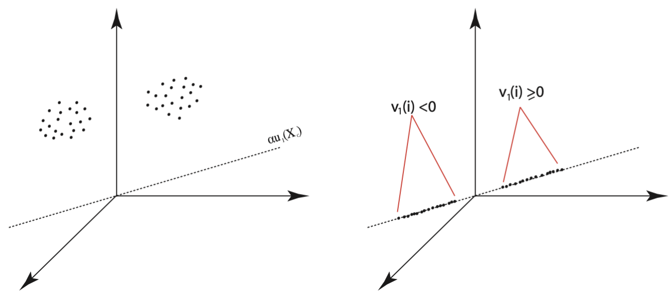
Figure 21.2: Illustration of Principal Direction Divisive Partitioning: Two Clusters and their Corresponding Projections on the First Principal Component
Once the data are divided, the two clusters are examined to find the one with the greatest variance (scatter). This subset of data is then extracted from the original data matrix, centered and projected onto the span of its own first principal component. The split at zero is made again and the algorithm proceeds iteratively until the desired number of clusters has been produced.
It is necessary to note, however, that the example in Figure 21.2 is truly an ideal geometric configuration of data. Figure 21.3 illustrates two configurations in which PDDP would fail. In the configuration on the left, both clusters would be split down the middle, and in the configuration on the right, the middle cluster would be split in the first iteration. Unfortunately, once data points are separated in an iteration of PDDP, there is no chance for them to be rejoined later. Table 21.1 provides the PDDP Algorithm.
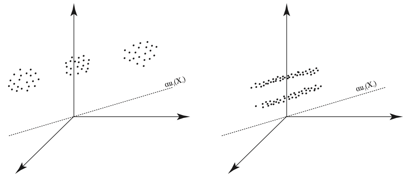
Figure 21.3: Failures of Principal Direction Divisive Partitioning: Two Configurations of Data that would be Poorly Clustered by PDDP
|
Since its initial publication, variations of the PDDP algorithm have been proposed, most notably PDDP(\(\ell\)) [59] and KPDDP [4], both developed by Dimitrios Zeimpekis and Efstratios Gallopoulos from the University of Patras in Greece. PDDP(\(\ell\)) uses the sign patterns in the first \(\ell\) principal components to partition the data into at most \(2^\ell\) clusters at each step of the algorithm, whereas KPDDP is a kernel variant which uses \(k\)-means to steer the cluster assignments at each step.
21.2 Iterative Partitional Algorithms
Iterative partitional algorithms begin with an initial partition of the data into \(k\) clusters and iteratively update the cluster memberships according to some notion of what constitutes a ``better" partition [42], [43]. The \(k\)-means algorithm is one example of a partitional algorithm. Before we get into the details of the modern day \(k\)-means algorithms, we’ll take a look back at the history that fostered its development as one of the best-known and most widely used clustering algorithms in the world.
21.2.1 Early Partitional Algorithms
Although the name ``\(k\)-means" was first used by MacQueen in 1967 [39], the partitional method generally referred to by this name today was proposed by Forgy in 1965 [40]. Forgy’s algorithm involves iteratively updating \(k\) seed points which, at each pass of the algorithm, define a partitioning of the data by associating each data point with its nearest seed point. The seeds are then updated to represent the centroids (means) of the resulting clusters and the process is repeated. Euclidean distance is the most common metric for measuring the nearness of points in these algorithms, but other metrics, such as Mahalanobis distance and angular distance, can and have been used as well. \(K\)-means can also handle binary or categorical variables by using simple matching coefficients found in the data mining literature, for example [67]. Forgy’s method is outlined in Table 21.2.
|
In 1966, Jancey suggested a variation of this method where the new seeds points in step 2 were computed by reflecting the old seed point across the new centroid, as depicted in Figure 21.4. Jancey argued that the data’s nearness to point 1 grouped them into a cluster initially, and thus using a seed point which exaggerates this movement toward the new centroid ought to help speed up convergence, and possibly lead to a better solution by avoiding local minima [38].
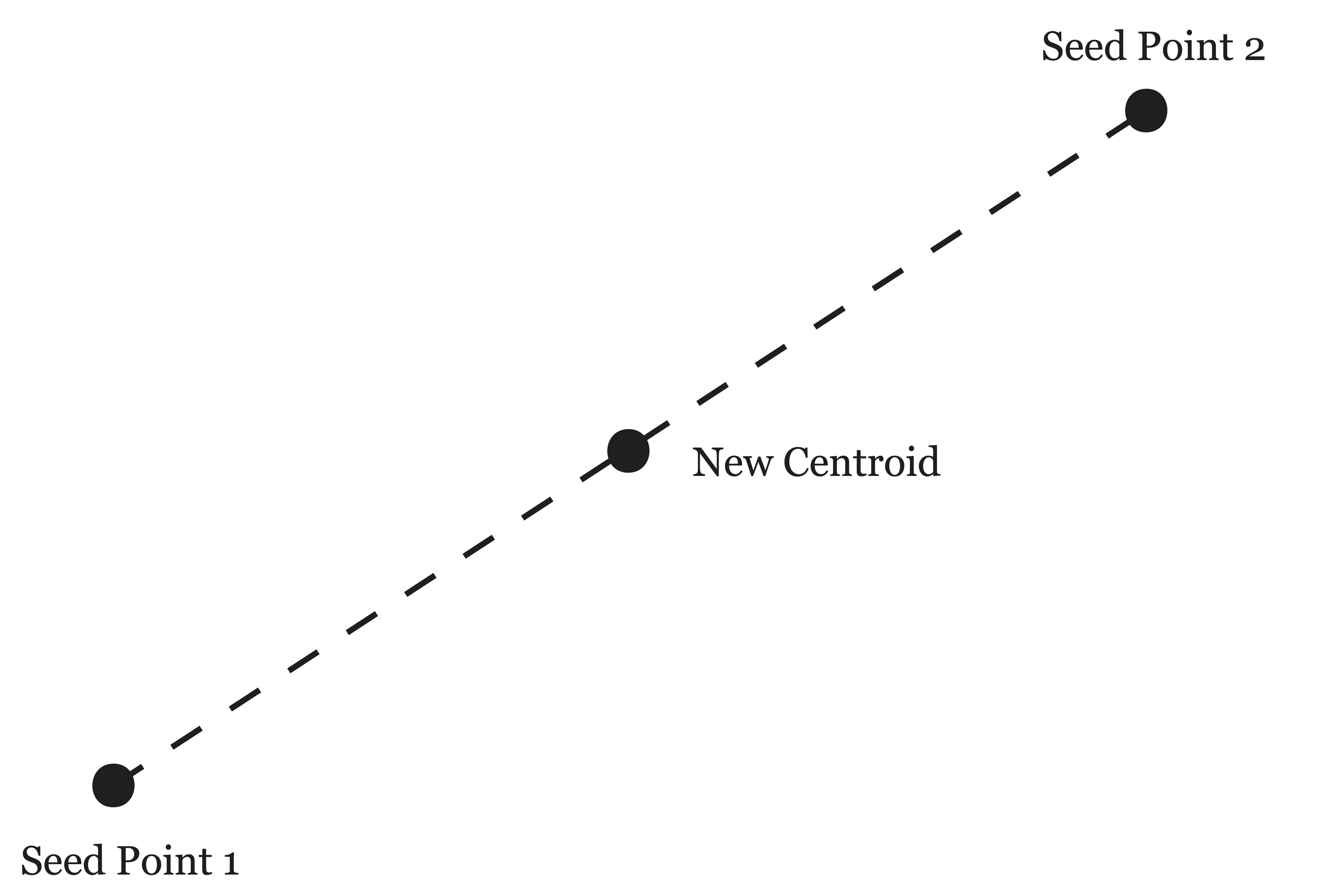
Figure 21.4: Jancey’s method of reflecting old seed point across the centroid to determine new seed point
MacQueen’s 1967 partitional process, which he called ``\(k\)-means", differs from Forgy’s formulation in that it a) specifies initial seed points and b) assigns data points to clusters one-by-one, updating the seed to be the centroid of the cluster each time a new point is added. The algorithm only makes one pass through the data. MacQueen’s method is presented in Table 21.3.
Input: \(n\) data points
|
As you can see, MacQueen’s algorithm, while similar in spirit, is quite different from that proposed by Forgy. The set of clusters found is likely to be dependent upon the order of the data, a property generally undesirable in cluster analysis. MacQueen stated that in his experience, these discrepancies in final solution based upon the order of the data were generally minor, and thus not unlike those caused by the choice of initialization in Forgy’s method. An advantage of MacQueen’s algorithm is the reduced computation load achieved by avoiding the continual processing of the data to convergence. It has also been suggested that MacQueen’s method may be useful to initialize the seeds for Forgy’s algorithm [43] and in fact this option is available in many data mining software packages like SAS’s Enterprise Miner.
Discussion of some additional partitional methods, including Dubes and Jain’s FORGY implementation and Ball and Hall’s ISODATA algorithm, is deferred to Chapter ?? because they involve procedures aimed at determining the number of clusters in the data.
21.2.2 \(k\)-means
We will finish our discussion of \(k\)-means with what has become the classical presentation. We begin with a matrix of column data, \(\X=[\mathbf{x}_1,\mathbf{x}_2,\dots,\mathbf{x}_n]\) where \(\mathbf{x}_i \in \Re^m, 1 \leq i \leq n\). The objective of \(k\)-means is to determine a partitioning of the data into \(k\) sets, \(C=\{C_1, C_2, \dots, C_k\}\), such that an intra-cluster sum of squares cost function is minimized: \[ \mbox{arg}\min_C \sum_{i=1}^{k} \sum_{\mathbf{x}_j \in C_i} \|\bo{x}_j-\boldsymbol \mu_i \|^2 \] Any desired distance metric can be used, according to the applications and whims of the user. Euclidean distance is standard, and leads to the specification Euclidean \(k\)-means. In document clustering, it is common to use the cosine of the angle between two data vectors (documents) to measure their distance from each other. This variant is commonly referred to as spherical \(k\)-means and will be discussed briefly in Section 21.2.2.1. The \(k\)-means algorithm, which is essentially the same as Forgy’s algorithm in Section 21.2, is presented in Table 21.4.
Input: Data points \(\{\mathbf{x}_1,\mathbf{x}_2,\dots,\mathbf{x}_n\}\) and set of initial centroids \(\{\boldsymbol \mu_1^{(0)},\boldsymbol \mu_2^{(0)},\dots, \boldsymbol \mu_k^{(0)}\}\).
|
This algorithm is guaranteed to converge because there are a finite number of partitions possible and at each pass of the algorithm the intra-cluster sum of squares cost function is decreased due to the fact that points are reassigned to a new cluster only if they are closer to the existing centroid of the new cluster than they were to the old one. The cost function is further reduced as the new centroids are calculated and the process repeats, lowering the cost function at each step. However, it is quite common for the algorithm to converge to local minima, particularly with large datasets. The output of \(k\)-means is sensitive to the initialization of the centroids and the choice of distance metric used in step 2. Randomly initialized centroids tend to be the most popular, but one can also seed the algorithm with centroids of clusters determined by another clustering algorithm.
21.2.2.1 Spherical \(k\)-means
In some applications, such as document clustering, similarity is often measured by the cosine of the angle \(\theta\) between two objects \(\mathbf{x}_i\) and \(\mathbf{x}_j\) (each normalized to have unit norm), \[\cos(\theta)=\mathbf{x}_i^T\mathbf{x}_j.\] This similarity is often transformed into a distance by computing the quantity \(d(\mathbf{x}_i,\mathbf{x}_j)=1-\cos(\theta)\) to formulate the spherical \(k\)-means objective function as follows: \[\min_C \sum_{i=1}^k \sum_{\mathbf{x} \in C_i} 1- \mathbf{x}^T \bo{c}_i.\] Where $_i = _i $ is the normalized centroid of the cluster. The spherical \(k\)-means algorithm is the same as the euclidean \(k\)-means algorithm aside from the definition of nearness in step 2.
21.2.2.2 \(k\)-mediods: Partitioning around Mediods (PAM) and Clustering Large Applications (CLARA)
In 1987, Kaufman and Rousseeuw devised another partitional method which searched through data in order to find \(k\) representative points (or mediods) belonging to the dataset which would serve as cluster centers in the same way the centroids do in \(k\)-means. They called these points ``representative" because it was thought the points would give some interpretability to the groups by exhibiting some defining characteristics of their associated clusters and distinguishing characteristics from other clusters. The authors’ original algorithm, Partitioning around Mediods (PAM), was not suitable for large datasets because of the computation time necessary to search through the data points to build the set of \(k\) representative points. The same authors developed a second algorithm, Clustering Large Applications (CLARA), to combat this problem. The central idea of CLARA was to use PAM on large datasets by sampling the data and applying the algorithm on the smaller sample. Once \(k\) representative points were found in the sample, the remaining data were associated with the mediod to which they were closest. The quality of the clustering is measured by the average distance of every object to its representative point. Five such samples are drawn, and the clustering that results in the lowest average distance is retained [35].
21.2.3 The Expectation-Maximization (EM) Clustering Algorithm
The Expectation-Maximization (EM) Algorithm, originally proposed by Dempster, Laird, and Rubin in 1977 [34], is one that has been used to solve many types of statistical problems over the years. It is generally used to determine parameters of a statistical model used to describe observations in a dataset. Here we will show how the algorithm is used for clustering, as in [33]. Our discussion is limited to the variant of the algorithm which uses Gaussian mixtures to model the data.
Supposing that our data points, \(\mathbf{x}_1,\mathbf{x}_2,\dots,\mathbf{x}_n\), each belonging to one of \(k\) clusters (or classes), \(C_1,C_2,\dots, C_k\). Then there exists some latent variables \(y_i, \,\, 1\leq i\leq n\), which identify the class membership of each \(\mathbf{x}_i\). It is assumed that each class label \(C_i\) determines the probability distribution of the data in that class. Here, we assume that this distribution is multivariate Gaussian. The parameters of this model include the a priori probabilities of each of the \(k\) classes, \(P(C_i)\), and the parameters of the corresponding normal distributions \(\boldsymbol \mu_i\) and \(\mathbf{\Sigma_i}\), which are the mean and covariance matrix respectively. The objective of the EM algorithm is to determine the parameters which maximize the likelihood of the data: \[\log L = \sum_i (\log P(y_i) + \log P(\mathbf{x}_i|y_i))\]
The EM algorithm takes as input a set of \(m\)-dimensional data points, \(\{\mathbf{x}_i\}_{i=1}^n\), the desired number of clusters \(k\), and an initial set of parameters \(\theta_j\) for each cluster \(C_j\) \(1\leq j\leq k\). For Guassian mixtures, \(\theta_j\) consists of mean \(\boldsymbol \mu_j\) and an \(m\times m\) covariance matrix \(\mathbf{\Sigma_j}\). The a priori probability of each cluster, \(\alpha_j = P(C_j)\) must also be initialized and updated throughout the algorithm. If no information is known about the underlying clusters, then we suggest initialization \(\alpha_j = 1/k\) for all clusters \(C_j\). EM then operates by iteratively executing an expectation step, where the probability that each data point belongs to each of the \(k\) classes is computed, followed by a maximization step, where the parameters for each class are updated to maximize the likelihood of the data [33]. These steps are summarized in Table 21.5.
Input: \(n\) data points, \(\{\mathbf{x}_i\}_{i=1}^n\), number of clusters \(k\), and initial set of parameters for each cluster \(C_j\): \(\alpha_j\) and \(\theta_j = \{\boldsymbol \mu_j, \Sigma_j\}\,\,1\leq j\leq k\)
|
The EM Algorithm with Gaussian mixtures works well for clustering when the normality assumption of the underlying clusters holds true. Unfortunately, it is difficult to know if this is the case prior to the identification of the clusters. The algorithm suffers considerable computational drawbacks, particularly with regards to storage of the \(k\) covariance matrices \(\mathbf{\Sigma_j}\in \Re^{m\times m}\), and is not easily run in parallel. For this reason, the EM algorithm is generally limited in its ability to be used on large datasets, particularly when the number of attributes \(m\) is very large, as it is in document clustering.
21.3 Density Search Algorithms
If objects are depicted as data points in a metric space, then one may interpret the problem of clustering as an attempt to find areas of the space that are densely populated by points, separated by less populated areas. A natural approach to the problem is then to search through the space seeking these dense regions. Such algorithms have been referred to as density search algorithms [23]. While these algorithms tend to suffer on real data in both accuracy efficiency, their ability to identify noise and to estimate the number of clusters \(k\) makes them worthy of discussion.
Many density search algorithms have their roots in the single-linkage hierarchical algorithms described in Section 21.1. Individual points are joined together in clusters one-by-one based upon their similarity (or nearness in space). However in this case there exists some criteria for which objects are rejected from joining an existing cluster and instead are set out to form their own cluster. For example, suppose we had two distinct well separated dense regions of points. Beginning with a single point in the first region, we form a cluster and search through the remaining points one by one adding them to the cluster in they satisfy some specified criterion of nearness to the points already in the cluster. Once all the points in the first region are combined into a single cluster, the purpose of the criterion is to reject points from the second region from joining the first cluster, causing them to create a new cluster.
The conception of density search algorithms dates to the late `60s with the taxmap method of Carmichael et al. in [21], [22] and the mode analysis method of Wishart [20]. In taxmap the authors suggested criterion like the drop in average similarity upon adding a new point to a cluster. In mode analysis the criterion was simply containment in a specified radius of points in a cluster. The problem with this approach was that it had trouble finding both large and small clusters simultaneously [23].
All density search algorithms suffer from the inability to find clusters of varying density, no matter how the term is defined in application, because the density of points is used to define the notion of a cluster. High dimensional data adds to this problem as demonstrated in Chapter ?? because as the size of the space grows, the points naturally become less and less dense inside of it. Another problem with density search algorithm is the necessity to search through data again and again, making their implementation difficult if not irrelevant for large data sets. Among the benefits to these methods are the inherent estimation of the number of clusters and their ability to find irregularly shaped (non-convex) clusters. Several algorithms in this category, like Density Based Spacial Clustering of Applications with Noise (DBSCAN) also make an effort to determine outliers or noise in the data. Because of the computational workload of these methods, we will abandon them after the present discussion in favor of more efficient methods. For an in-depth analysis of other density search algorithms and their variants, see [19].
21.3.1 Density Based Spacial Clustering of Applications with Noise (DBSCAN)
Density Based Spacial Clustering of Applications with Noise (DBSCAN) is an algorithm proposed by Ester, Kriegel, Sander, and Xu in 1996 [18], which uses the Euclidean nearness of a group of points in \(m\)-space to define density. The algorithm uses the terminology in Definition 21.1.
Definition 21.1 (DBSCAN Terms) The following definitions will aid our discussion of the DBSCAN algorithm:
Dense Point and \(\rho_{min}\): A point \(\mathbf{x}_j\) is called dense if there are at least \(\rho_{min}\) other points contained in its \(\epsilon\)-neighborhood.
Direct Density Reachability: A point \(\mathbf{x}_i\) is called directly density reachable from a point \(\mathbf{x}_j\) if it is in the \(\epsilon\)-neighborhood surrounding \(\mathbf{x}_j\), i.e. if \(\mathbf{x}_i \in \mathscr{N}(\mathbf{x}_j,\epsilon)\), and \(\mathbf{x}_j\) is a dense point.
Density Reachability: A point \(\mathbf{x}_i\) is called density reachable from a point \(\mathbf{x}_j\) if there is a sequence of points \(\mathbf{x}_{1},\mathbf{x}_{2},\dots, \mathbf{x}_{p}\) with \(\mathbf{x}_{1}=\mathbf{x}_j\) and \(\mathbf{x}_{p}=\mathbf{x}_i\) where each \(\mathbf{x}_{{k+1}}\) is directly density reachable from \(\mathbf{x}_{k}.\)
Noise Point: A point \(\mathbf{x}_l\) is called a noise point or outlier if it contains 0 points in its \(\epsilon\)-neighborhood.
The relationship of density reachability is not symmetric. This fact is illustrated in Figure 21.5. A point in this illustration is dense if its \(\epsilon\)-neighborhood contains at least \(\rho_{min} = 2\) other points. The green point \(a\) is density reachable from the blue point \(b\), however the reverse is not true because \(a\) is not a dense point. Because of this, we introduce the notion of density connectedness.
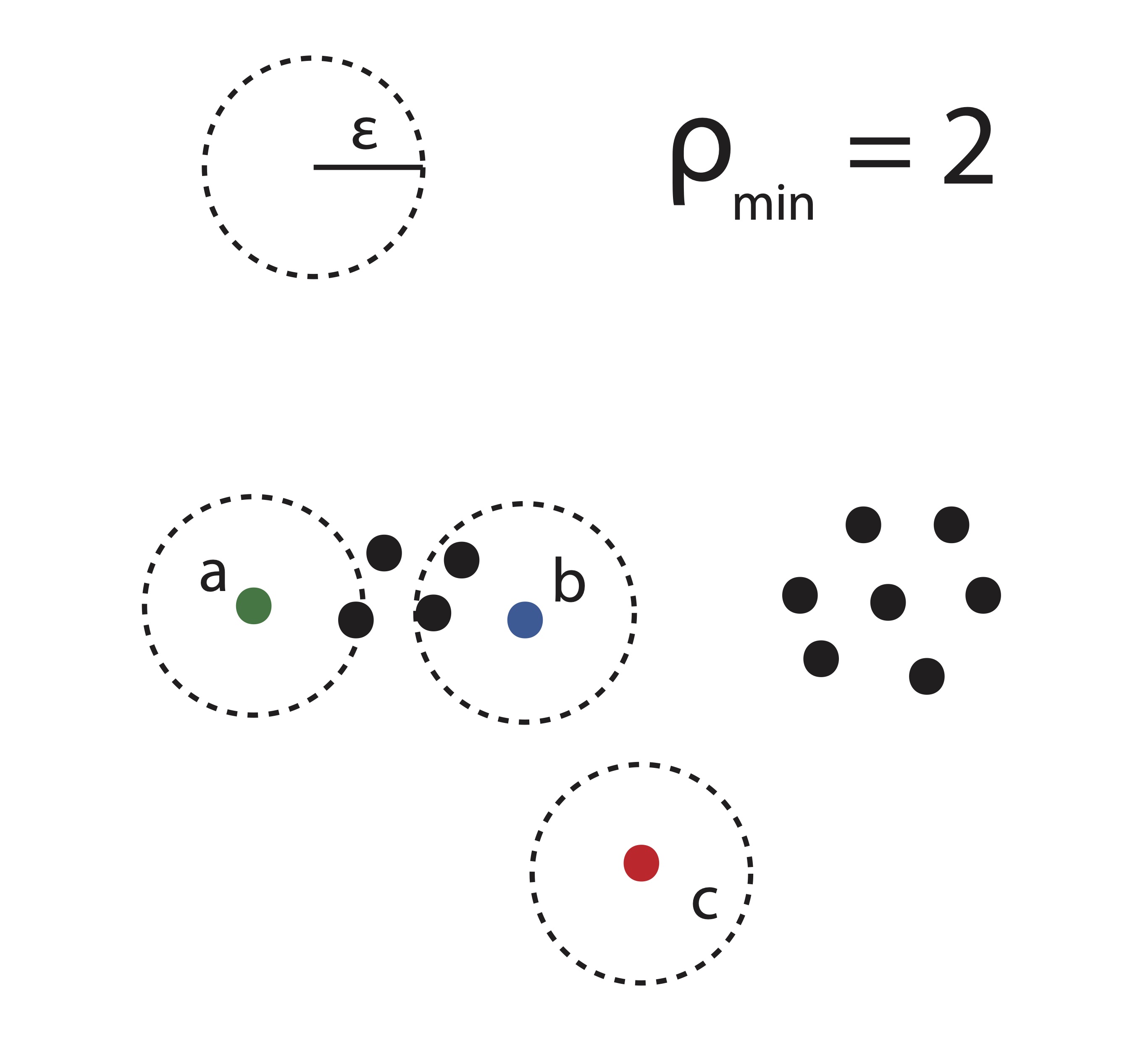
Figure 21.5: DBSCAN Illustration
Definition 21.2 (Density Connectedness) Two points \(\mathbf{x}_i\) and \(\mathbf{x}_j\) are density-connected if there exists some point \(\mathbf{x}_k\) such that both \(\mathbf{x}_i\) and \(\mathbf{x}_j\) are density reachable from \(x_k\).
In Figure 21.5, it is clear that we can say points \(a\) and \(b\) are density-connected since they are each density reachable from any of the 4 points in between them. The point \(c\) in this illustration is a noise point or outlier because there are no points contained in its \(\epsilon\)-neighborhood.
Using these definitions, we can formalize the properties that define a cluster in DBSCAN.
Definition 21.3 (DBSCAN Cluster) Given the parameters \(\rho_{min}\) and \(\epsilon\), a DBSCAN cluster is a set of points that satisfy the two following conditions:
- All points within the cluster are mutually density-connected.
- If a point is density-connected to any point in the cluster, it is part of the cluster as well.
Table 21.6 describes how DBSCAN finds such clusters.
Input: Set of points \(\mathbf{X}=[\mathbf{x}_1,\mathbf{x}_2,\dots,\mathbf{x}_n]\) to be clustered and parameters \(\epsilon\) and \(\rho_{min}\)
Output: Clusters found \(C_1,\dots,C_k\) |
21.4 Conclusion
The purpose of this chapter was to give the reader a basic understanding of hierarchical, iterative partitional, and density search approaches to data clustering. One of the main concerns addressed in this paper is that all of these algorithms have merit, but in application rarely do the algorithms completely agree on a solution. In fact, algorithms with random inputs like \(k\)-means are not even likely to agree with themselves over a number of different trials. It can be extremely difficult to qualitatively measure the goodness of your clustering when the data cannot be visualized in 2 or 3 dimensions. While there are a number of metrics to help the user get a sense of the compactness of the clusters (see Chapter 23), the effect of noise and outliers can often blur the true picture. It is also common for such metrics to take nearly equivalent values for vastly different cluster solutions, forcing the user to choose a solution using domain knowledge and utility. First we will look at another class of clustering methods which aim to solve the graph partitioning problem described in Chapter ??.
The difference between the problems of data clustering and graph partitioning is merely the structure of the input objects to be clustered. In data clustering, the input objects are composed of measurements on \(m\) variables or features. If we interpret the graph partitioning problem in such a way that input objects are vertices on a graph and the variables describing them are the weights of the edges by which they are connected to other vertices, then it becomes clear we can use any of the methods in this chapter to cluster the columns of an adjacency matrix as described in Chapter ??. Similarly if one creates a similarity matrix for objects from a data clustering problem, we can cluster that matrix using the theory and algorithms from graph partitioning. While each problem can be transformed into the other, the design of the algorithms for the two cases is generally quite different. In the next chapter, we provide a thorough overview of some popular graph clustering algorithms.