Chapter 10 Least Squares
10.1 Introducing Error
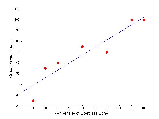
The least squares problem arises in almost all areas of applied mathematics. In data science, the idea is generally to find an approximate mathematical relationship between predictor and target variables such that the sum of squared errors between the true target values and the predicted target values is minimized. In two dimensions, the goal would be to develop a line as depicted in Figure 10.1 such that the sum of squared vertical distances (the residuals, in green) between the true data (in red) and the mathematical prediction (in blue) is minimized.
Figure 10.1: Least Squares Illustrated in 2 dimensions
If we let \(\bo{r}\) be a vector containing the residual values \((r_1,r_2,\dots,r_n)\) then the sum of squared residuals can be written in linear algebraic notation as \[\sum_{i=1}^n r_i^2 = \bo{r}^T\bo{r}=(\y-\hat{\y})^T(\y-\hat{\y}) = \|\y-\hat{\y}\|^2\]
Suppose we want to regress our target variable \(\y\) on \(p\) predictor variables, \(\x_1,\x_2,\dots,\x_p\). If we have \(n\) observations, then the ideal situation would be to find a vector of parameters \(\boldsymbol\beta\) containing an intercept, \(\beta_0\) along with \(p\) slope parameters, \(\beta_1,\dots,\beta_p\) such that \[\begin{equation} \tag{10.1} \underbrace{\bordermatrix{1&\x_1 & \x_2 & \dots & \x_p}{obs_1\\obs_2\\ \vdots \\ obs_n}{\left(\begin{matrix} 1 & x_{11} & x_{12} & \dots & x_{1p}\\ 1 & x_{21} & x_{22} & \dots & x_{2p}\\ \vdots & \vdots & \vdots & \vdots &\vdots\\ 1 & x_{n1} & x_{n2} & \dots & x_{np} \end{matrix}\right) }}_{\LARGE\mathbf{X}} \underbrace{\left(\begin{matrix} \beta_0\\ \beta_1\\ \vdots \\ \beta_p \end{matrix}\right)}_{\LARGE \boldsymbol\beta} = \underbrace{\pm y_0\\ y_1 \\ \vdots \\ y_n \mp}_{\LARGE \y} \end{equation}\]
With many more observations than variables, this system of equations will not, in practice, have a solution. Thus, our goal becomes finding a vector of parameters \(\hat{\bbeta}\) such that \(\X\hat{\bbeta}=\hat{\y}\) comes as close to \(\y\) as possible. Using the design matrix, \(\X\), the least squares solution \(\hat{\boldsymbol\beta}\) is the one for which \[\|\y-\X\hat{\boldsymbol\beta} \|^2=\|\y-\hat{\y}\|^2\] is minimized. Theorem 10.1 characterizes the solution to the least squares problem.
Theorem 10.1 (Least Squares Problem and Solution) For an \(n\times m\) matrix \(\X\) and \(n\times 1\) vector \(\y\), let \(\bo{r} = \X\widehat{\boldsymbol\beta} - \y\). The least squares problem is to find a vector \(\widehat{\boldsymbol\beta}\) that minimizes the quantity \[\sum_{i=1}^n r_i^2 = \|\y-\X\widehat{\boldsymbol\beta} \|^2.\]
Any vector \(\widehat{\bbeta}\) which provides a minimum value for this expression is called a least-squares solution.
- The set of all least squares solutions is precisely the set of solutions to the so-called normal equations, \[\X^T\X\widehat{\bbeta} = \X^T\y.\]
- There is a unique least squares solution if and only if \(rank(\X)=m\) (i.e. linear independence of variables or no perfect multicollinearity!), in which case \(\X^T\X\) is invertible and the solution is given by \[\widehat{\bbeta} = (\X^T\X)^{-1}\X^T\y\]
| ID | % of Exercises | Exam Grade |
| 1 | 20 | 55 |
| 2 | 100 | 100 |
| 3 | 90 | 100 |
| 4 | 70 | 70 |
| 5 | 50 | 75 |
| 6 | 10 | 25 |
| 7 | 30 | 60 |
To find the least squares regression line, we want to solve the equation \(\X\bbeta = \y\): \[ \pm 1 & 20\\ 1 & 100\\ 1 & 90\\ 1 & 70\\ 1 & 50\\ 1 & 10\\ 1 & 30\mp \pm \beta_0 \\ \beta_1 \mp = \pm 55\\100\\100\\70\\75\\25\\60 \mp \]
This system is obviously inconsistent. Thus, we want to find the least squares solution \(\hat{\bbeta}\) by solving \(\X^T\X\hat{\bbeta}=\X^T\y\):
\[\begin{eqnarray} \small \pm 1&1&1&1&1&1&1 \\20&100&90&70&50&10&30 \mp\pm 1 & 20\\ 1 & 100\\ 1 & 90\\ 1 & 70\\ 1 & 50\\ 1 & 10\\ 1 & 30\mp \pm \beta_0 \\ \beta_1 \mp &=&\pm 1&1&1&1&1&1&1 \\20&100&90&70&50&10&30 \mp \pm 55\\100\\100\\70\\75\\25\\60 \mp \cr \pm 7 & 370\\370&26900 \mp \pm \beta_0 \\ \beta_1 \mp &=& \pm 485 \\ 30800\mp \end{eqnarray}\]
Now, since multicollinearity was not a problem, we can simply find the inverse of \(\X^T\X\) and multiply it on both sides of the equation: \[\pm 7 & 370\\370&26900 \mp^{-1}= \pm 0.5233 & -0.0072\\ -0.0072 & 0.0001 \mp\] and so \[\pm \beta_0 \\ \beta_1 \mp = \pm 0.5233 & -0.0072\\ -0.0072 & 0.0001 \mp \pm 485 \\ 30800\mp = \pm 32.1109 \\0.7033\mp\]
Thus, for each additional 10% of exercises completed, exam grades are expected to increase by about 7 points. The data along with the regression line \[grade=32.1109+0.7033percent\_exercises\] is shown below.
:::
10.2 Why the normal equations?
The normal equations can be derived using matrix calculus (demonstrated at the end of this section) but the solution of the normal equations also has a nice geometrical interpretation. It involves the idea of orthogonal projection, a concept which will be useful for understanding future topics.
10.2.1 Geometrical Interpretation
In order for a system of equations, \(\A\x=\b\) to have a solution, \(\b\) must be a linear combination of columns of \(\A\). That is simply the definition of matrix multiplication and equality. If \(\A\) is \(m\times n\) then \[\A\x=\b \Longrightarrow \b = x_1\A_1+x_2\A_2+\dots+x_n\A_n.\] As discussed in Chapter 7, another way to say this is that \(\b\) is in the \(span\) of the columns of \(\A\). The \(span\) of the columns of \(\A\) is called the column space of \(\A\). In Least-Squares applications, the problem is that \(\b\) is not in the column space of \(\A\). In essence, we want to find the vector \(\hat{\b}\) that is closest to \(\b\) but exists in the column space of \(\A\). Then we know that \(\A\hat{\x}=\hat{\b}\) does have a unique solution, and that the right hand side of the equation comes as close to the original data as possible. By multiplying both sides of the original equation by \(\A^T\) what we are really doing is projecting \(\b\) orthogonally onto the column space of \(\A\). We should think of the column space as a flat surface (perhaps a plane) in space, and \(\b\) as a point that exists off of that flat surface. There are many ways to draw a line from a point to plane, but the shortest distance would always be travelled perpendicular (orthogonal) to the plane. You may recall from undergraduate calculus or physics that a normal vector to a plane is a vector that is orthogonal to that plane. The normal equations, \(\A^T\A\x=\A^T\b\), help us find the closest point to \(\b\) that belongs to the column space of \(\A\) by means of an orthogonal projection. This geometrical vantage point is depicted in Figure 10.2.
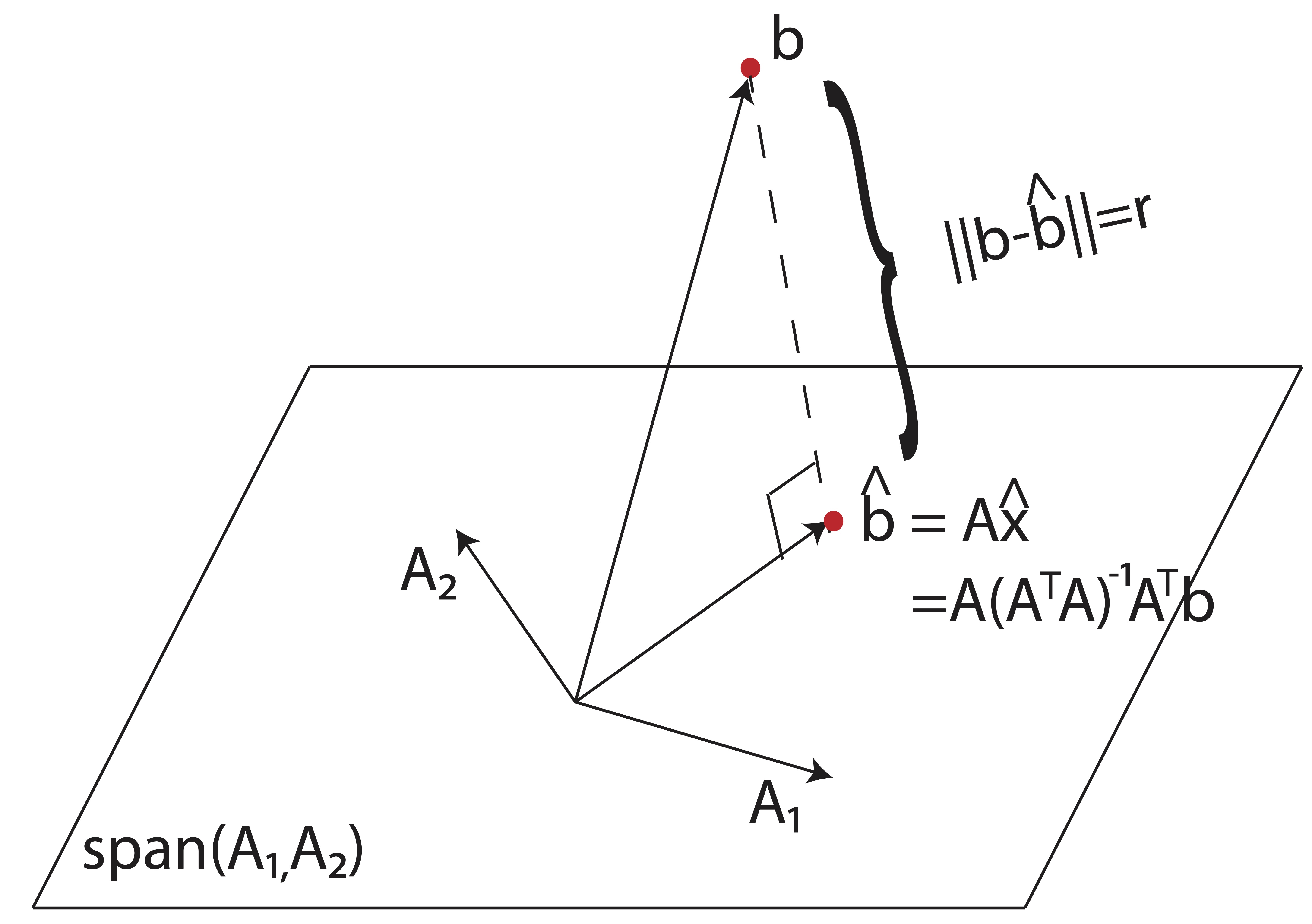
Figure 10.2: The normal equations yield the vector \(\hat{\b}\) in the column space of \(\A\) which is closest to the original right hand side \(\b\) vector.
10.2.2 Calculus Derivation
If you’ve taken a course in undergraduate calculus, you recall that finding minima and maxima of functions typically involves taking their derivatives and setting them equal to zero. That approach to the derivation of the normal equations will be fruitful, but we first need to understand how to take derivatives of matrix equations. Without teaching vector calculus, we will simply provide the following required formulas for matrix derivatives. If you’ve taken some undergraduate calculus, perhaps you’ll see some parallels.
While \(\frac{\partial}{\partial \mathbf{x}}\) would commonly be the formula reported, we’ve swapped out the \(\mathbf{x}\) for \(\boldsymbol \beta\) in the table below in an effort to make our current problem more recognizable.
| Condition | Formula |
| \(\mathbf{a}\) is not a function of \(\boldsymbol \beta\) | \(\frac{\partial \mathbf{a}}{\partial \boldsymbol \beta}= \mathbf{0}\) |
| \(\mathbf{a}\) is not a function of \(\boldsymbol \beta\) | \(\frac{\partial \boldsymbol \beta}{\partial \boldsymbol \beta}= \mathbf{I}\) |
| \(\A\) is not a function of \(\boldsymbol \beta\) | \(\frac{\partial \boldsymbol \beta^T\mathbf{A}}{\partial \boldsymbol \beta}= \mathbf{A}^T\) |
| \(\A\) is not a function of \(\boldsymbol \beta\) | \(\frac{\partial \boldsymbol \beta^T\mathbf{A}\boldsymbol \beta}{\partial \boldsymbol \beta}= (\mathbf{A}+\mathbf{A}^T)\boldsymbol \beta\) |
|
\(\A\) is not a function of \(\boldsymbol \beta\) \(\A\) is symmetric | \(\frac{\partial \boldsymbol \beta^T\mathbf{A}\boldsymbol \beta}{\partial \boldsymbol \beta}= 2\mathbf{A}\boldsymbol \beta\) |
Now let’s start with our objective, which is to minimize sum of squared error, by writing it as the inner product of the vector of residuals with itself: \[\boldsymbol \varepsilon^T \boldsymbol \varepsilon = (\mathbf{y}-\mathbf{X}\boldsymbol \beta)^T(\mathbf{y}-\mathbf{X}\boldsymbol \beta)\] We’d like to minimize this function with respect to \(\boldsymbol \beta\), our vector of unknowns. Thus, our procedure will be to take the derivative with respect to \(\boldsymbol \beta\) and set it equal to 0. Note, on the second line of this proof, we take advantage of the fact that \(\mathbf{a}^T\mathbf{b} = \mathbf{b}^T\mathbf{a}\) for all \(\mathbf{a},\mathbf{b} \in \Re^n\)
\[\begin{eqnarray*} \frac{\partial}{\partial \boldsymbol \beta} \left(\boldsymbol \varepsilon^T \boldsymbol \varepsilon\right) &=& \frac{\partial}{\partial \boldsymbol \beta} \left(\mathbf{y}^T\mathbf{y} - \mathbf{y}^T(\mathbf{X}\boldsymbol \beta) - (\mathbf{X}\boldsymbol \beta)^T\mathbf{y} + (\mathbf{X}\boldsymbol \beta)^T(\mathbf{X}\boldsymbol \beta)\right)\\ &=& \frac{\partial}{\partial \boldsymbol \beta} \left(\mathbf{y}^T\mathbf{y} -2\mathbf{y}^T(\mathbf{X}\boldsymbol \beta) + \boldsymbol \beta\mathbf{X}^T\mathbf{X} \boldsymbol \beta \right)\\ &=& 0 - 2\mathbf{X}^Ty + 2\mathbf{X}^T\mathbf{X}\boldsymbol \beta \end{eqnarray*}\]
Setting the last line equal to zero and solving for \(\boldsymbol \beta\) completes the derivation. \(\Box\)
In Chapter 11, we’ll take a deeper dive into the utility of least squares for applied data science.