Chapter 20 Introduction
Clustering is the task of partitioning a set of objects into subsets (clusters) so that objects in the same cluster are similar in some sense. Thus, a “cluster” is a generally a subjective entity determined by how an observer defines the similarity of objects. Take for example Figure 20.1 where we depict eight objects that differ by shape and color. Depending on the notion of similarity used (color, shape, or both) these objects might be clustered in one of the three ways shown.
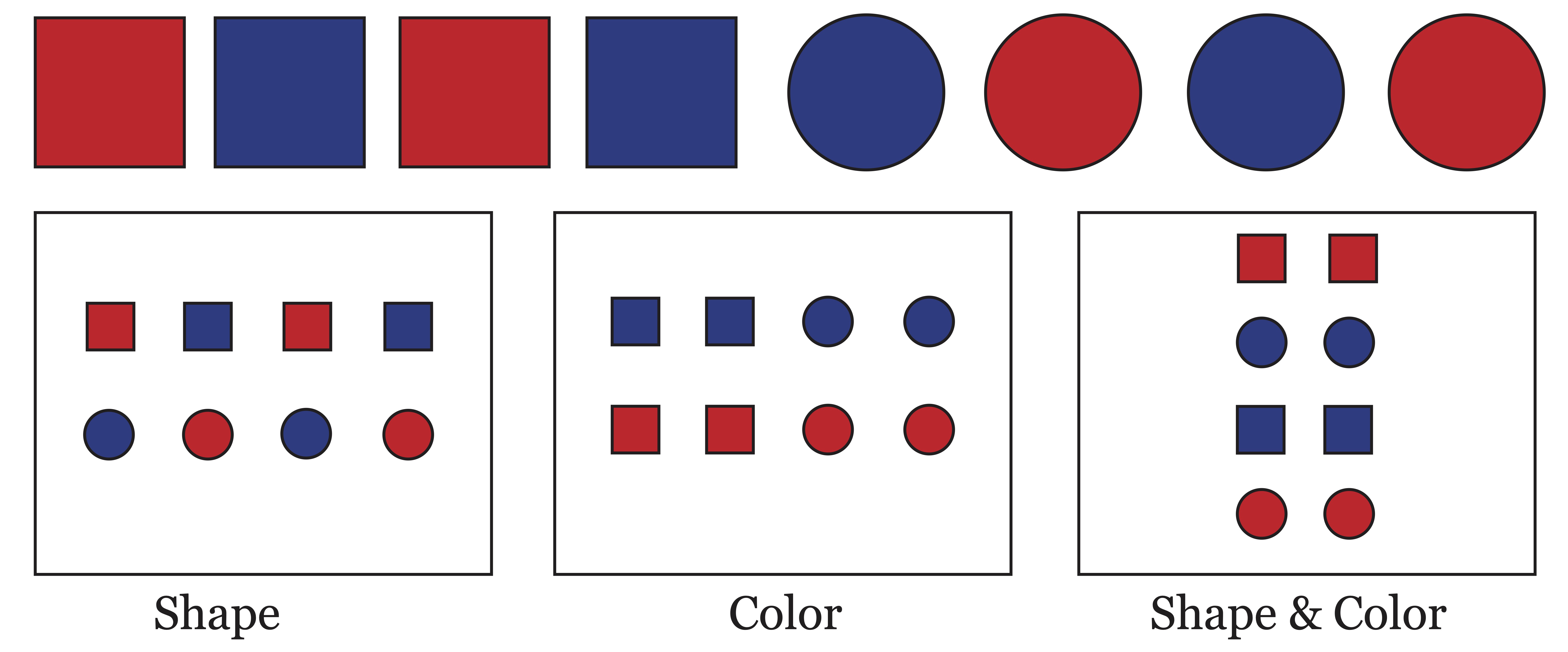
Figure 20.1: Three Meaningful Clusterings of One Set of Objects
20.1 Mathematical Setup
In order to define this problem in a mathematical sense, it is necessary to quantify the attributes of objects using data so that we can mathematically or statistically determine notions of similarity. Data clustering refers to the process of grouping data points naturally based on information found in the data which describes its characteristics and relationships. It is not an exact science and, as we will discuss at length, there is no best method for partitioning data into clusters.
20.1.1 Data
We will use the terms “observation,” “object,” and “data point” interchangeably to refer to the entities we aim to partition into clusters. These data points could represent any population of interest, be it a collection of documents or a group of Iris flowers. Each data point will be considered as a column vector, containing measurements of features, attributes, or variables (again, used interchangeably) which characterize it. For example, a column vector characterizing a document could have as many rows as there are words in the dictionary, and each entry in the vector could indicate the number of times each word occurred in the document. An Iris flower, on the other hand, may be characterized by far fewer attributes, perhaps measurements on the size of its petal and sepal. It is assumed we have \(n\) such objects, each represented by a column vector \(\x_j\) containing measurements on \(m\) variables. All of this information is collected in an \(m \times n\) data matrix, \(\X\), which will serve as input to the various clustering methods. \[\X=[\x_1,\x_2,\dots,\x_n]\]
The aim of data clustering is to automatically determine clusters in these populations based upon the information contained in those vectors. In the document collection, the goal may be to identify clusters of documents which discuss similar subject matter whereas in the Iris data, the goal may be to learn about different species of Iris flowers.
In applied data mining, variables fall into the following four categories: Nominal/Categorical, Ordinal, Interval, or Ratio.- Nominal/Categorical: Variables which have no ordering, for example ethnicity, color or shape.
- Ordinal: Variables which can be rank-ordered but for which distances have no meaning. For example, scores assigned to levels education (0=no high school, 1=some high school, 2=high school diploma). The distance between 0 and 1 is not necessarily the same as the distance between 1 and 2, but the numbers have some meaning by order.
- Interval: Variables for which differences can be interpreted but for with ratios make no sense. For example if temperature is measured in degrees Fahrenheit the distance from 20 to 30 degrees is the same as the distance from 70 to 80 degrees, however 80 degrees is not ``twice as hot’’ as 40 degrees.
- Ratio: variables for which a meaningful ratio can be constructed. For example height or weight. An absolute zero is meaningful for a ratio variable.
For the algorithms contained herein, it is assumed that the attributes used are ratio variables, although many of the methods can be extended to include other types of data (or one can simply use dummy variables and/or ordinal encoding as long as one explores the potential impacts of such decisions).
20.2 The Number of Clusters, \(k\)
One of the important problems in cluster analysis is the determination of the number of clusters, \(k\). The number of clusters can also be a matter of subjectivity. Take for instance the 2-dimensional scatter plot of points in Figure 20.2. Using the points’ proximity in Euclidean space as a measure of their similarity, one could argue that there are any number of clusters in this simple illustration. However, most people would agree that there is indeed cluster-like structure in this data.
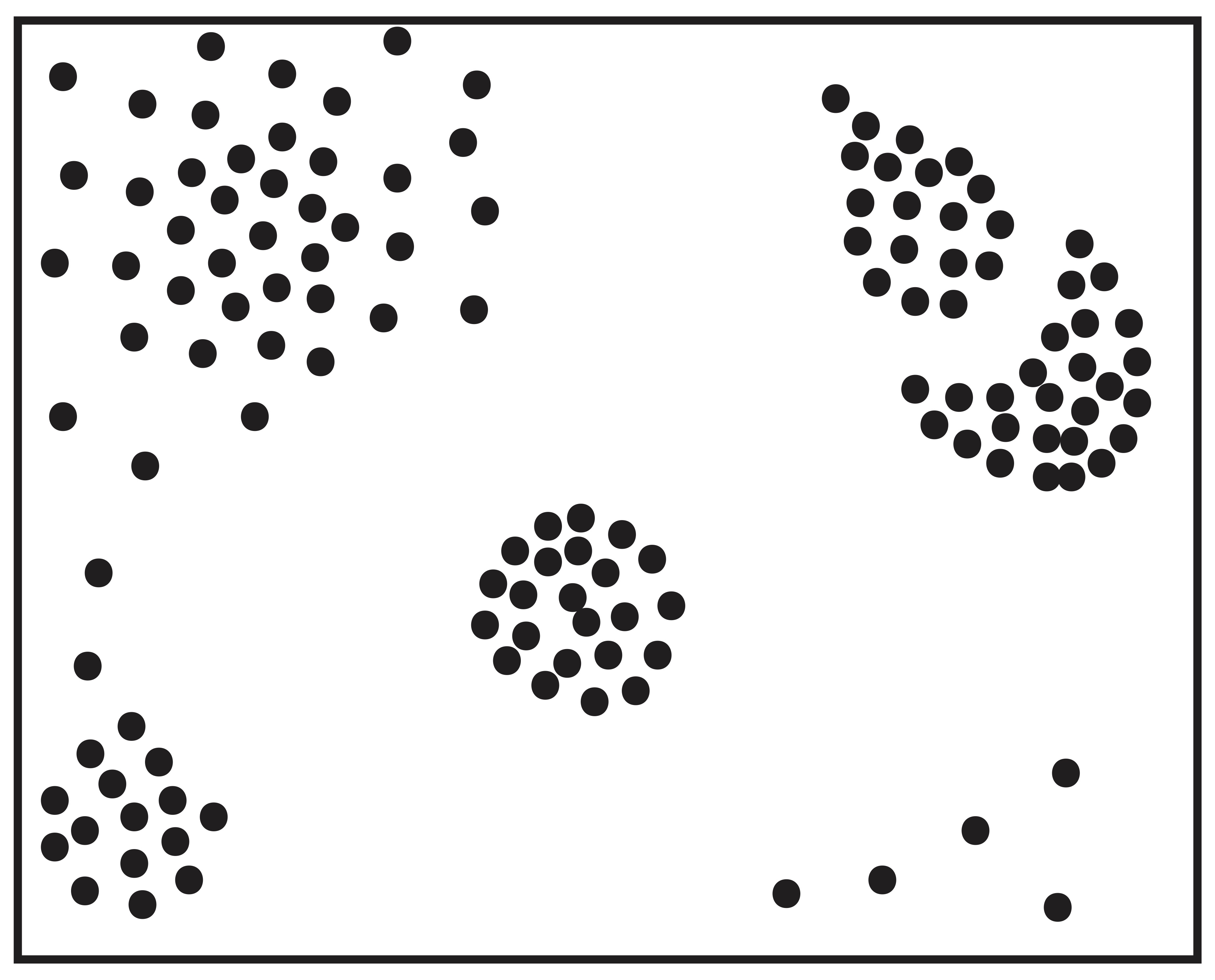
Figure 20.2: How Many Clusters do You See?
Figure 20.2 also motivates a discussion of subcluster structure. Figure 20.3 shows two possible clusterings with different numbers of clusters. The clustering on the right depicts a logical subdivison of the clusters on the left.
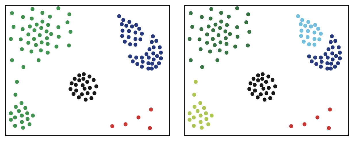
Figure 20.3: Two Reasonable Answers with Different Numbers of Clusters
It is easy to imagine data in which the number of clusters to specify is a matter of debate only because groups of related objects can be meaningfully divided into subcategories or subclusters. For example a collection of webpages may clearly fall into 3 categories: sports, investment banking, and astronomy. If the webpages about sports further divide into 2 categories like baseball and basketball then we’d refer to that as subclustering.
20.3 Partitioning of Graphs and Networks
Another popular research problem in clustering is the partitioning of graphs. In network applications this problem has become known to many as community detection [63], although the underlying problem of partitioning graphs has been studied extensively for years [26]–[28], [31], [58], [61], [71]. A graph is a set of vertices (or equivalently nodes) \(V=\{1,2,\dots, n\}\) together with a set of edges \(E=\{(i,j) : i,j \in V\}\) which connect vertices together. A weighted graph is one in which the edges are assigned some weight \(w_{ij}\) whereas an unweighted graph has binary weights for edges: \(w_{ij}=1\) if \((i,j) \in E\), \(w_{ij}=0\) otherwise. Our focus will be on undirected graphs in which \(w_{ij}=w_{ji}\). All algorithms for graph partitioning (or network community detection) will rely on an adjacency matrix.
Definition 20.1 (Adjacency Matrix) An adjacency matrix \(\A\) for an undirected graph, \(\mathcal{G}=(V,E)\), is an \(n \times n\) symmetric matrix defined as follows: \[\A_{ij}= \begin{cases} w_{ij}, & \text{if } (i,j) \in E \\ 0 & \text{otherwise} \end{cases}\]
Figure 20.4 is an example of a graph exhibiting cluster or community structure. The weights of the edges are depicted by their thickness. It is expected that edges within the clusters occur more frequently and with higher weight than edges between the clusters. Thus, once the rows and columns of the matrix are reordered according to their cluster membership, we expect to see a matrix that is block-diagonally dominant - that is, one in which values in square diagonal blocks are relatively large compared to those in the off-diagonal blocks.
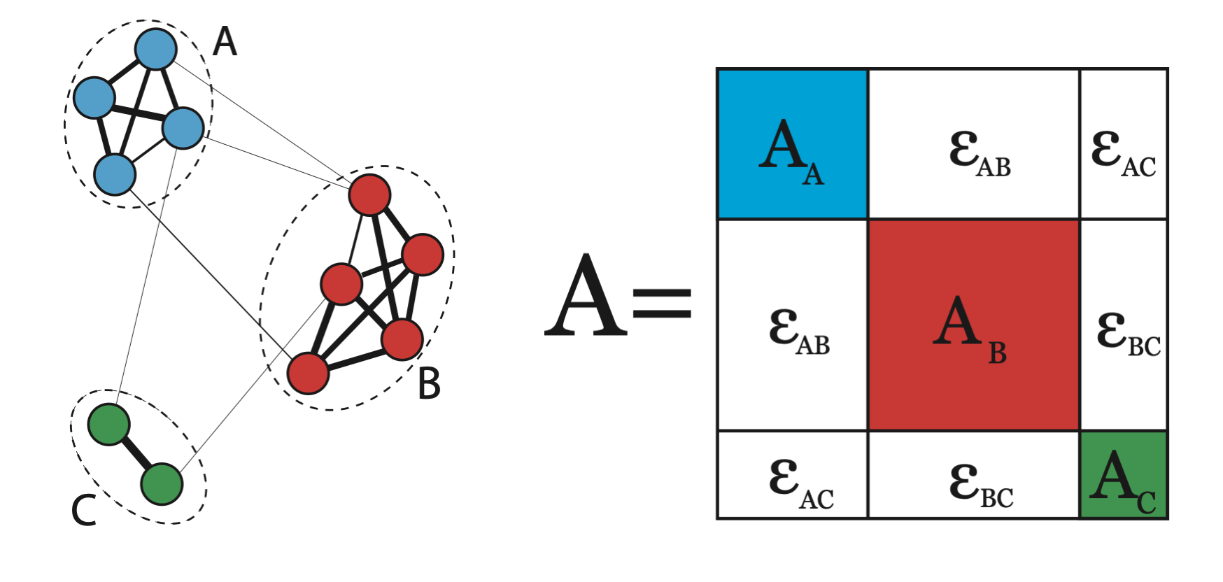
Figure 20.4: A Graph with Clusters and its Block Diagonally Dominant Adjacency Matrix
In much of the literature on graph partitioning, it is suggested that the data clustering problem can be transformed into a graph partitioning problem by means of a similarity matrix [71]. A similarity matrix \(\bo{S}\) is an \(n \times n\) symmetric matrix where \(\bo{S}_{ij}\) measures some notion of similarity between data points \(\x_i\) and \(\x_j\). There are a wealth of metrics available to gauge similarity or dissimilarity, see for example [16]. Common measures of similarity rely on Euclidean or angular distance measures. Two of the most popular similarity functions in the literature are the following:
- Gaussian Similarity: \[\bo{S}_{ij} =\mbox{exp}(-\frac{\|\x_i-\x_j\|^2}{2\alpha^2})\] where \(\alpha\) is a tuning parameter.
- Cosine Similarity: \[\bo{S}_{ij}=\cos (\x_i,\x_j) = \frac{\x_i^T\x_j}{\|\x_i\|\|\x_j\|}\]
Any similarity matrix can be considered an adjacency matrix for a graph, thus transforming the original data clustering problem into a graph partitioning problem. Several algorithms for data clustering and graph partitioning are provided in Section 21. Regardless of the method chosen for clustering, similarity matrices can be a useful tool for visualizing cluster results in light of the block diagonal structure shown in Figure 20.4. This block diagonal structure can be visualized using a heat map of a similarity matrix. A matrix heat map represents each value in a matrix by a colored pixel indicating the magnitude of the value. Figure 20.5 is an example of a heat map using real data. The data are a collection of news articles (documents) from the web containing seven different topics of discussion. The rows and columns of the cosine similarity matrix for these documents have been reordered according to some cluster solution. White pixels represent negligible values of similarity. Some of these topics are closely related, which can be seen by the heightened level of similarities between blocks.
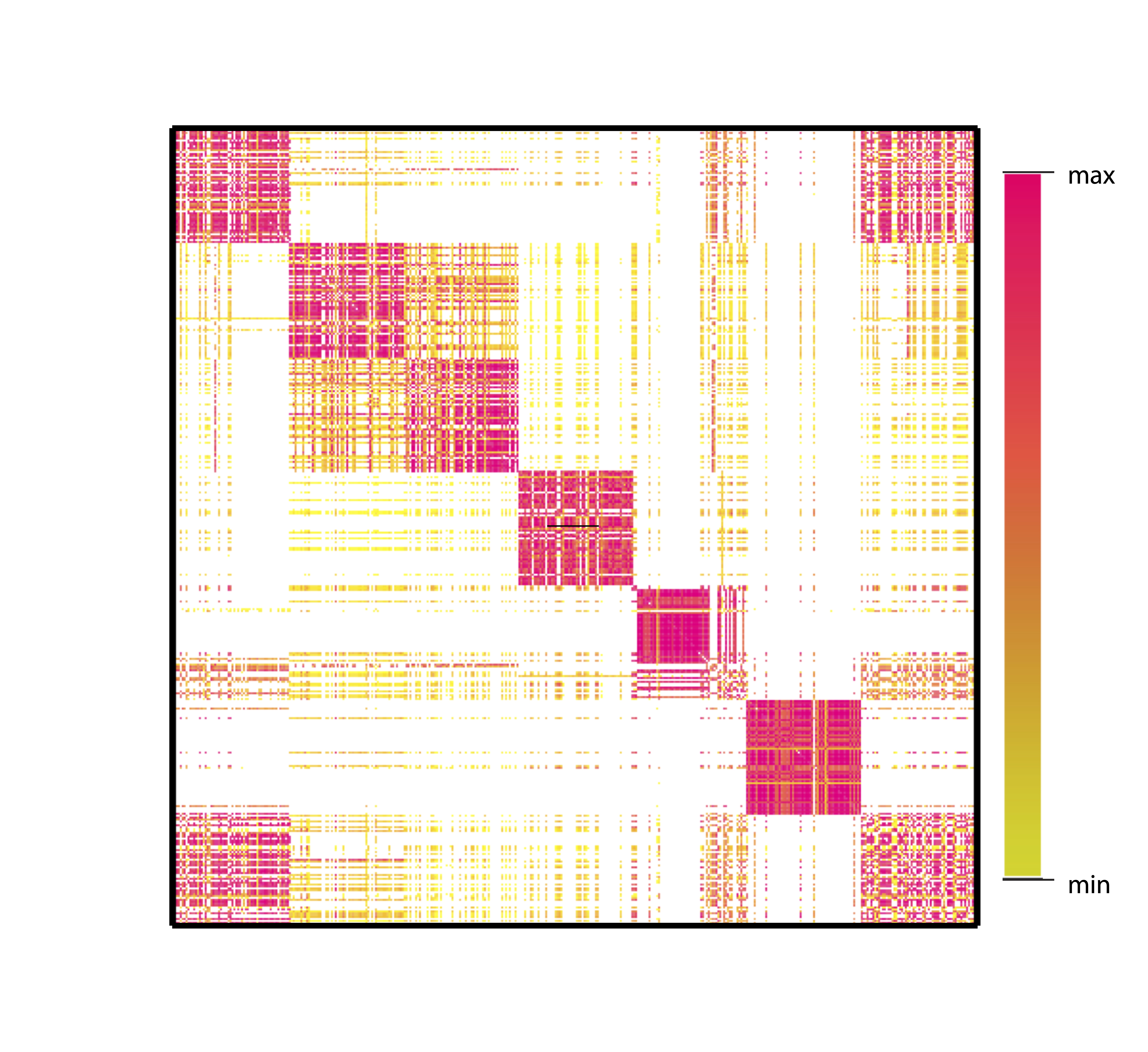
Figure 20.5: Heat Map of Similarity Matrix Exhibiting Cluster Structure
While a heat-map visualization allows the user to get a sense of the quality of a specific clustering, it does not always make it easy to determine which is a better solution given two different clusterings. Since clustering is an unsupervised process, quantitative measures of cluster quality are often used to compare different clusterings. A short survery of these metrics is given in Section 23. First, we will take a brief historical look at the roots of cluster analysis and how it emerged into a major field of research in the late twentieth century.
20.4 History of Data Clustering
According to Anil Jain in [50], data clustering first appeared in an article written by Forrest Clements in 1954 about anthropological data [49]. However, a Google Scholar search provides several earlier publications whose titles also contain the phrase “cluster analysis” [47]. In fact, the discussion of data clustering dates back to the 1930’s when anthropologists Driver and Kroeber [46] and psychologists Zubin [45] and Tryon [44] realized the utility of such analysis in determining cultural or psychological classifications. While the usefulness of such techniques was clear to researchers in many social and biological disciplines at that time, the lack of computational tools made the analysis time consuming and practically impossible for large sets of data.
Cluster analysis exploded into the limelight in the 1960’s and `70’s after Sokal and Sneath’s 1963 book Principles of Numerical Taxonomy [51]. Although the text is primarily geared toward biologists faced with the task of classifying organisms, it motivated researchers from many different disciplines to consider the problem of data clustering from other angles like computing, statistics, and domain specific applications. [25]. Sokal and Sneath’s book presents a detailed discussion of the simple, intuitive, and still popular hierarchical clustering (see Section 21.1) techniques for biological taxonomy. These authors also provided perhaps the earliest mention of the matrix heat map visualizations of clustering that are still popular today. Figure 20.6 shows an example of one of these heat maps, then drawn by hand, from their book.
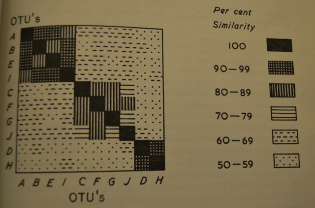
Figure 20.6: Hand Drawn Matrix Heat Map Visualization from 1963 Book by Sokal and Sneath
Prior to the development of modern computational resources, programs for numerical taxonomy were written in machine language and not easily transferred from one computer to another [51]. However, by the mid 1960s, it was clear that the advancement in technology would probably keep pace with advancements in algorithm design and many researchers from various disciplines began to contribute to the clustering literature. The following sections present an in-depth view of the most popular developments in data clustering since that time. Chapter ?? explores a common problem associated with the massive datasets of modern day.