Chapter 16 Applications of SVD
16.1 Text Mining
Text mining is another area where the SVD is used heavily. In text mining, our data structure is generally known as a Term-Document Matrix. The documents are any individual pieces of text that we wish to analyze, cluster, summarize or discover topics from. They could be sentences, abstracts, webpages, or social media updates. The terms are the words contained in these documents. The term-document matrix represents what’s called the “bag-of-words” approach - the order of the words is removed and the data becomes unstructured in the sense that each document is represented by the words it contains, not the order or context in which they appear. The \((i,j)\) entry in this matrix is the number of times term \(j\) appears in document \(i\).
Definition 16.1 (Term-Document Matrix) Let \(m\) be the number of documents in a collection and \(n\) be the number of terms appearing in that collection, then we create our term-document matrix \(\A\) as follows: \[\begin{equation} \begin{array}{ccc} & & \text{term 1} \quad \text{term $j$} \,\, \text{term $n$} \\ \A_{m\times n} = & \begin{array}{c} \hbox{Doc 1} \\ \\ \\ \hbox{Doc $i$} \\ \\ \hbox{Doc $m$} \\ \end{array} & \left( \begin{array}{ccccccc} & & & |& & & \\ & & & |& & & \\ & & & |& & & \\ & - & - &f_{ij} & & & \\ & & & & & & \\ & & & & & & \\ \end{array} \right) \end{array} \nonumber \end{equation}\] where \(f_{ij}\) is the frequency of term \(j\) in document \(i\). A binary term-document matrix will simply have \(\A_{ij}=1\) if term \(j\) is contained in document \(i\).
16.1.1 Note About Rows vs. Columns
You might be asking yourself, “Hey, wait a minute. Why do we have documents as columns in this matrix? Aren’t the documents like our observations?” Sure! Many data scientists insist on having the documents on the rows of this matrix. But, before you do that, you should realize something. Many SVD and PCA routines are created in a way that is more efficient when your data is long vs. wide, and text data commonly has more terms than documents. The equivalence of the two presentations should be easy to see in all matrix factorization applications. If we have \[\A = \U\mathbf{D}\V^T\] then, \[\A^T = \V\mathbf{D}\U^T\] so we merely need to switch our interpretations of the left- and right-singular vectors to switch from document columns to document rows.
Beyond any computational efficiency argument, we prefer to keep our documents on the columns here because of the emphasis placed earlier in this text regarding matrix multiplication viewed as a linear combination of columns. The animation in Figure 2.7 is a good thing to be clear on before proceeding here.
16.1.2 Term Weighting
Term-document matrices tend to be large and sparse. Term-weighting schemes are often used to downplay the effect of commonly used words and bolster the effect of rare but semantically important words . The most popular weighting method is known as Term Frequency-Inverse Document Frequency (TF-IDF). For this method, the raw term-frequencies \(f_{ij}\) in the matrix \(\A\) are multiplied by global weights called inverse document frequencies, \(w_i\), for each term. These weights reflect the commonality of each term across the entire collection and ultimately quantify a term’s ability to narrow one’s search results (the foundations of text analysis were, after all, dominated by search technology). The inverse document frequency of term \(i\) is:
\[w_i = \log \left( \frac{\mbox{total # of documents}}{\mbox{# documents containing term } i} \right)\]
To put this weight in perspective, for a collection of \(n=10,000\) documents we have \(0\leq w_j \leq 9.2\), where \(w_j=0\) means the word is contained in every document (rendering it useless for search) and \(w_j=9.2\) means the word is contained in only 1 document (making it very useful for search). The document vectors are often normalized to have unit 2-norm, since their directions (not their lengths) in the term-space is what characterizes them semantically.
16.1.3 Other Considerations
In dealing with text, we want to do as much as we can do minimize the size of the dictionary (the collection of terms which enumerate the rows of our term-document matrix) for both computational and practical reasons. The first effort we’ll make toward this goal is to remove so-called stop words, or very common words that appear in a great many sentences like articles (“a,” “an,” “the”) and prepositions (“about,” “for,” “at”) among others. Many projects also contain domain-specific stop words. For example, one might remove the word “Reuters” from a corpus of Reuters’ newswires. The second effort we’ll often make is to apply a stemming algorithm which reduces words to their stem. For example, the words “swimmer” and “swimming” would both be reduced to their stem, “swim.” Stemming and stop word removal can greatly reduce the size of the dictionary and also help draw meaningful connections between documents.
16.1.4 Latent Semantic Indexing
The noise-reduction property of the SVD was extended to text processing in 1990 by Susan Dumais et al, who named the effect Latent Semantic Indexing (LSI). LSI involves the singular value decomposition of the term-document matrix defined in Definition 16.1. In other words, it is like a principal components analysis using the unscaled, uncentered inner-product matrix \(\A^T\A\). If the documents are normalized to have unit length, this is a matrix of cosine similarities (see Chapter 6). Cosine similarity is the most common measure of similarity between documents for text mining. If the term-document matrix is binary, this is often called the co-occurrence matrix because each entry gives the number of times two words occur in the same document.
It certainly seems logical to view text data in this context as it contains both an informative signal and semantic noise. LSI quickly grew roots in the information retrieval community, where it is often used for query processing. The idea is to remove semantic noise, due to variation and ambiguity in vocabulary and presentation style, without losing significant amounts of information. For example, a human may not differentiate between the words “car” and “automobile,” but indeed the words will become two separate entities in the raw term-document matrix. The main idea in LSI is that the realignment of the data into fewer directions should force related documents (like those containing “car” and “automobile”) closer together in an angular sense, thus revealing latent semantic connections.
Purveyors of LSI suggest that the use of the Singular Value Decomposition to project the documents into a lower-dimensional space results in a representation which reflects the major associative patterns of the data while ignoring less important influences. This projection is done with the simple truncation of the SVD shown in Equation (15.3).
As we have seen with other types of data, the very nature of dimension reduction makes possible for two documents with similar semantic properties to be mapped closer together. Unfortunately, the mixture of signs (positive and negative) in the singular vectors (think principal components) makes the decomposition difficult to interpret. While the major claims of LSI are legitimate, this lack of interpretability is still conceptually problematic for some folks. In order to make this point as clear as possible, consider the original “term basis” representation for the data, where each document (from a collection containing \(m\) total terms in the dictionary) could be written as: \[\A_j = \sum_{i=1}^{m} f_{ij}\e_i\] where \(f_{ij}\) is the frequency of term \(i\) in the document, and \(\e_i\) is the \(i^{th}\) column of the \(m\times m\) identity matrix. The truncated SVD gives us a new set of coordinates (scores) and basis vectors (principal component features): \[\A_j \approx \sum_{i=1}^r \alpha_i \u_i\] but the features \(\u_i\) live in the term space, and thus ought to be interpretable as a linear combinations of the original “term basis.” However the linear combinations, having both positive and negative coefficients, tends to be semantically obscure in practice - These new features do not often form meaningful topics for the text, although they often do organize in a meaningful way as we will demonstrate in the next section.
16.1.5 Example
Let’s consider a corpus of short documents, perhaps status updates from social media sites. We’ll keep this corpus as minimal as possible to demonstrate the utility of the SVD for text.
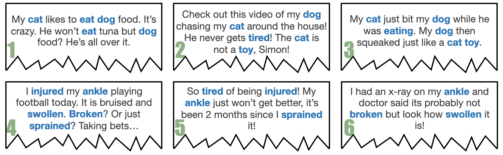
Figure 16.1: A corpus of 6 documents. Words occurring in more than one document appear in bold. Stop words removed, stemming utilized. Document numbers correspond to term-document matrix below.
\[\begin{equation*} \begin{array}{cc} & \begin{array}{cccccc} \;doc_1\; & \;doc_2\;& \;doc_3\;& \;doc_4\;& \;doc_5\;& \;doc_6\; \end{array}\\ \begin{array}{c} \hbox{cat} \\ \hbox{dog}\\ \hbox{eat}\\ \hbox{tired} \\ \hbox{toy}\\ \hbox{injured} \\ \hbox{ankle} \\ \hbox{broken} \\ \hbox{swollen} \\ \hbox{sprained} \\ \end{array} & \left( \begin{array}{cccccc} \quad 1\quad & \quad 2\quad & \quad 2\quad & \quad 0\quad & \quad 0\quad & \quad 0\quad \\ \quad 2\quad & \quad 3\quad & \quad 2\quad & \quad 0\quad & \quad 0\quad & \quad 0\quad \\ \quad 2\quad & \quad 0\quad & \quad 1\quad & \quad 0\quad & \quad 0\quad & \quad 0\quad \\ \quad 0\quad & \quad 1\quad & \quad 0\quad & \quad 0\quad & \quad 1\quad & \quad 0\quad \\ \quad 0\quad & \quad 1\quad & \quad 1\quad & \quad 0\quad & \quad 0\quad & \quad 0\quad \\ \quad 0\quad & \quad 0\quad & \quad 0\quad & \quad 1\quad & \quad 1\quad & \quad 0\quad \\ \quad 0\quad & \quad 0\quad & \quad 0\quad & \quad 1\quad & \quad 1\quad & \quad 1\quad \\ \quad 0\quad & \quad 0\quad & \quad 0\quad & \quad 1\quad & \quad 0\quad & \quad 1\quad \\ \quad 0\quad & \quad 0\quad & \quad 0\quad & \quad 1\quad & \quad 0\quad & \quad 1\quad \\ \quad 0\quad & \quad 0\quad & \quad 0\quad & \quad 1\quad & \quad 1\quad & \quad 0\quad \\ \end{array}\right) \end{array} \end{equation*}\]
We’ll start by entering this matrix into R. Of course the process of parsing a collection of documents and creating a term-document matrix is generally more automatic. The tm text mining library is recommended for creating a term-document matrix in practice.
A=matrix(c(1,2,2,0,0,0,
           2,3,2,0,0,0,
           2,0,1,0,0,0,
           0,1,0,0,1,0,
           0,1,1,0,0,0,
           0,0,0,1,1,0,
           0,0,0,1,1,1,
           0,0,0,1,0,1,
           0,0,0,1,0,1,
           0,0,0,1,1,0),
         nrow=10, byrow=T)
A
## [,1] [,2] [,3] [,4] [,5] [,6]
## [1,] 1 2 2 0 0 0
## [2,] 2 3 2 0 0 0
## [3,] 2 0 1 0 0 0
## [4,] 0 1 0 0 1 0
## [5,] 0 1 1 0 0 0
## [6,] 0 0 0 1 1 0
## [7,] 0 0 0 1 1 1
## [8,] 0 0 0 1 0 1
## [9,] 0 0 0 1 0 1
## [10,] 0 0 0 1 1 0Because our corpus is so small, we’ll skip the step of term-weighting, but we will normalize the documents to have equal length. In other words, we’ll divide each document vector by its two-norm so that it becomes a unit vector:
A_norm = apply(A, 2, function(x){x/c(sqrt(t(x)%*%x))})
A_norm
## [,1] [,2] [,3] [,4] [,5] [,6]
## [1,] 0.3333333 0.5163978 0.6324555 0.0000000 0.0 0.0000000
## [2,] 0.6666667 0.7745967 0.6324555 0.0000000 0.0 0.0000000
## [3,] 0.6666667 0.0000000 0.3162278 0.0000000 0.0 0.0000000
## [4,] 0.0000000 0.2581989 0.0000000 0.0000000 0.5 0.0000000
## [5,] 0.0000000 0.2581989 0.3162278 0.0000000 0.0 0.0000000
## [6,] 0.0000000 0.0000000 0.0000000 0.4472136 0.5 0.0000000
## [7,] 0.0000000 0.0000000 0.0000000 0.4472136 0.5 0.5773503
## [8,] 0.0000000 0.0000000 0.0000000 0.4472136 0.0 0.5773503
## [9,] 0.0000000 0.0000000 0.0000000 0.4472136 0.0 0.5773503
## [10,] 0.0000000 0.0000000 0.0000000 0.4472136 0.5 0.0000000We then compute the SVD of A_norm and observe the left- and right-singular vectors. Since the matrix \(\A\) is term-by-document, you might consider the terms as being the “units” of the rows of \(\A\) and the documents as being the “units” of the columns. For example, \(\A_{23}=2\) could logically be interpreted as “there are 2 units of the word dog per document number 3.” In this mentality, any factorization of the matrix should preserve those units. Similar to any “Change of Units Railroad”, matrix factorization can be considered in terms of units assigned to both rows and columns:
\[\A_{\text{term} \times \text{doc}} = \U_{\text{term} \times \text{factor}}\mathbf{D}_{\text{factor} \times \text{factor}}\V^T_{\text{factor} \times \text{doc}}\]
Thus, when we examine the rows of the matrix \(\U\), we’re looking at information about each term and how it contributes to each factor (i.e. the “factors” are just linear combinations of our elementary term vectors); When we examine the columns of the matrix \(\V^T\), we’re looking at information about how each document is related to each factor (i.e. the documents are linear combinations of these factors with weights corresponding to the elements of \(\V^T\)). And what about \(\mathbf{D}?\) Well, in classical factor analysis the matrix \(\mathbf{D}\) is often combined with either \(\U\) or \(\V^T\) to obtain a two-matrix factorization. \(\mathbf{D}\) describes how much information or signal from our original matrix exists along each of the singular components. It is common to use a screeplot, a simple line plot of the singular values in \(\mathbf{D}\), to determine an appropriate rank for the truncation in Equation (15.3).
out = svd(A_norm)
plot(out$d, ylab = 'Singular Values of A_norm')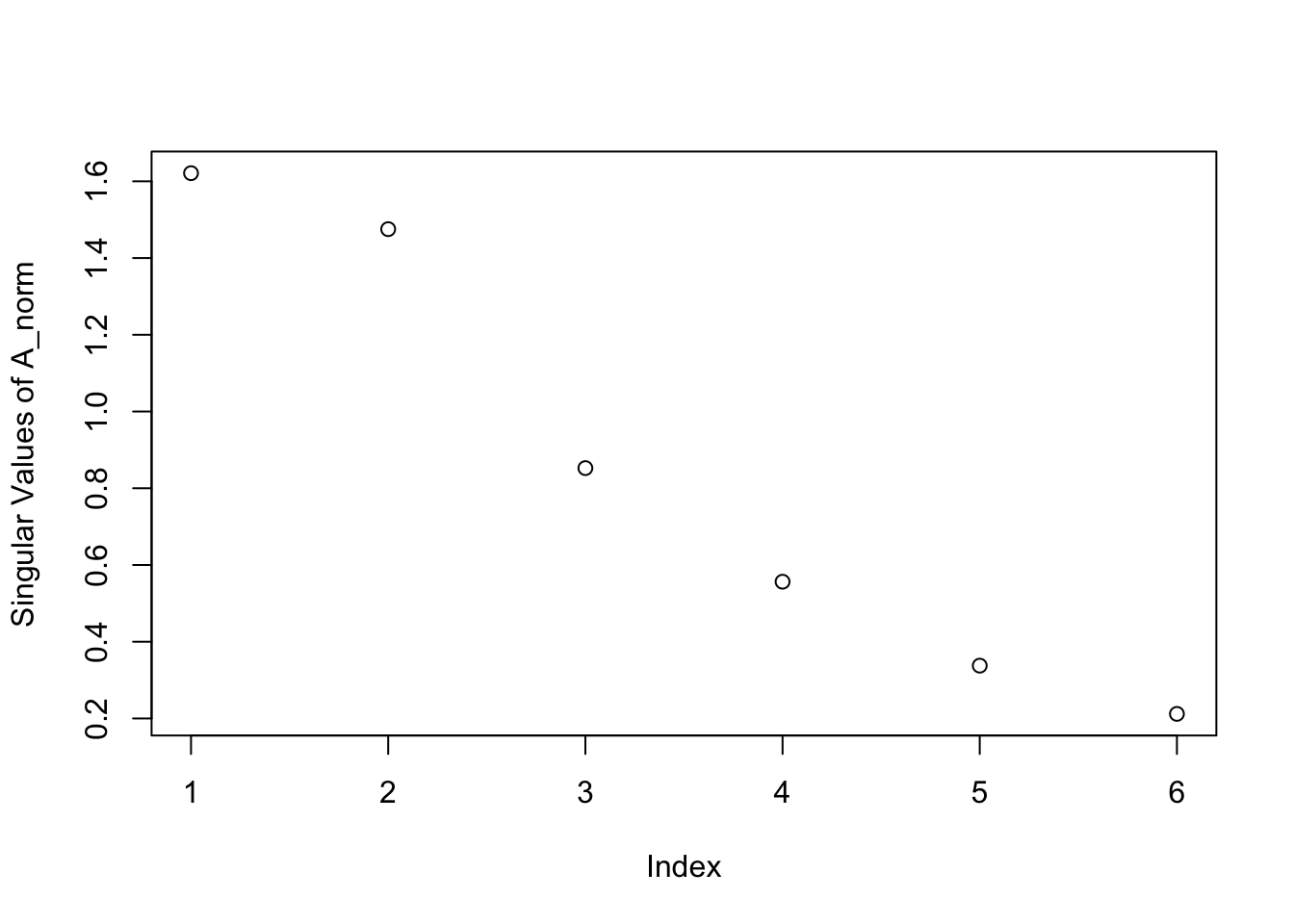
Figure 16.2: Screeplot for the Toy Text Dataset
Noticing the gap, or “elbow” in the screeplot at an index of 2 lets us know that the first two singular components contain notably more information than the components to follow - A major proportion of pattern or signal in this matrix lies long 2 components, i.e. there are 2 major topics that might provide a reasonable approximation to the data. What’s a “topic” in a vector space model? A linear combination of terms! It’s just a column vector in the term space! Let’s first examine the left-singular vectors in \(\U\). Remember, the rows of this matrix describe how the terms load onto factors, and the columns are those mysterious “factors” themselves.
out$u## [,1] [,2] [,3] [,4] [,5] [,6]
## [1,] -0.52980742 -0.04803212 0.01606507 -0.24737747 0.23870207 0.45722153
## [2,] -0.73429739 -0.06558224 0.02165167 -0.08821632 -0.09484667 -0.56183983
## [3,] -0.34442976 -0.03939120 0.10670326 0.83459702 -0.14778574 0.25277609
## [4,] -0.11234648 0.16724740 -0.47798864 -0.22995963 -0.59187851 -0.07506297
## [5,] -0.20810051 -0.01743101 -0.01281893 -0.34717811 0.23948814 0.42758997
## [6,] -0.03377822 0.36991575 -0.41154158 0.15837732 0.39526231 -0.10648584
## [7,] -0.04573569 0.58708873 0.01651849 -0.01514815 -0.42604773 0.38615891
## [8,] -0.02427277 0.41546131 0.45839081 -0.07300613 0.07255625 -0.15988106
## [9,] -0.02427277 0.41546131 0.45839081 -0.07300613 0.07255625 -0.15988106
## [10,] -0.03377822 0.36991575 -0.41154158 0.15837732 0.39526231 -0.10648584So the first “factor” of SVD is as follows:
\[\text{factor}_1 = -0.530 \text{cat} -0.734 \text{dog}-0.344 \text{eat}-0.112 \text{tired} -0.208 \text{toy}-0.034 \text{injured} -0.046 \text{ankle}-0.024 \text{broken} -0.024 \text{swollen} -0.034 \text{sprained} \] We can immediately see why people had trouble with LSI as a topic model – it’s hard to intuit how you might treat a mix of positive and negative coefficients in the output. If we ignore the signs and only investigate the absolute values, we can certainly see some meaningful topic information in this first factor: the largest magnitude weights all go to the words from the documents about pets. You might like to say that negative entries mean a topic is anticorrelated with that word, and to some extent this is correct. That logic works nicely, in fact, for factor 2:
\[\text{factor}_2 = -0.048\text{cat}-0.066\text{dog}-0.039\text{eat}+ 0.167\text{tired} -0.017\text{toy} 0.370\text{injured}+ 0.587\text{ankle} +0.415\text{broken} + 0.415\text{swollen} + 0.370\text{sprained}\] However, circling back to factor 1 then leaves us wanting to see different signs for the two groups of words. Nevertheless, the information separating the words is most certainly present. Take a look at the plot of the words’ loadings along the first two factors in Figure 16.3.
Figure 16.3: Projection of the Terms onto First two Singular Dimensions
Moving on to the documents, we can see a similar clustering pattern in the columns of \(\V^T\) which are the rows of \(\V\), shown below:
out$v## [,1] [,2] [,3] [,4] [,5] [,6]
## [1,] -0.55253068 -0.05828903 0.10665606 0.74609663 -0.2433982 -0.2530492
## [2,] -0.57064141 -0.02502636 -0.11924683 -0.62022594 -0.1219825 -0.5098650
## [3,] -0.60092838 -0.06088635 0.06280655 -0.10444424 0.3553232 0.7029012
## [4,] -0.04464392 0.65412158 0.05781835 0.12506090 0.6749109 -0.3092635
## [5,] -0.06959068 0.50639918 -0.75339800 0.06438433 -0.3367244 0.2314730
## [6,] -0.03357626 0.55493581 0.63206685 -0.16722869 -0.4803488 0.1808591In fact, the ability to separate the documents with the first two singular vectors is rather magical here, as shown visually in Figure 16.4.
Figure 16.4: Projection of the Docuemnts onto First two Singular Dimensions
Figure 16.4 demonstrates how documents that live in a 10-dimensional term space can be compressed down to 2-dimensions in a way that captures the major information of interest. If we were to take that 2-truncated SVD of our term-document matrix and multiply it back together, we’d see an approximation of our original term-document matrix, and we could calculate the error involved in that approximation. We could equivalently calculate that error by using the singular values.
A_approx = out$u[,1:2]%*% diag(out$d[1:2])%*%t(out$v[,1:2])
# Sum of element-wise squared error
(norm(A-A_approx,'F'))^2
## [1] 24.44893# Sum of squared singular values truncated
(sum(out$d[3:6]^2))## [1] 1.195292However, multiplying back to the original data is not generally an action of interest to data scientists. What we are after in the SVD is the dimensionality reduced data contained in the columns of \(\V^T\) (or, if you’ve created a document-term matrix, the rows of \(\U\).
16.2 Image Compression
While multiplying back to the original data is not generally something we’d like to do, it does provide a nice illustration of noise-reduction and signal-compression when working with images. The following example is not designed to teach you how to work with images for the purposes of data science. It is merely a nice visual way to see what’s happening when we truncate the SVD and omit these directions that have “minimal signal.”
16.2.1 Image data in R
Let’s take an image of a leader that we all know and respect:
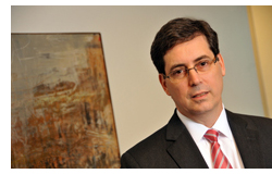
Figure 16.5: Michael Rappa, PhD, Founding Director of the Institute for Advanced Analytics and Distinguished Professor at NC State
This image can be downloaded from the IAA website, after clicking on the link on the left hand side “Michael Rappa / Founding Director.”
Let’s read this image into R. You’ll need to install the pixmap package:
#install.packages("pixmap")
library(pixmap)
Download the image to your computer and then set your working directory in R as the same place you have saved the image:
setwd("/Users/shaina/Desktop/lin-alg")The first thing we will do is examine the image as an [R,G,B] (extension .ppm) and as a grayscale (extension .pgm). Let’s start with the [R,G,B] image and see what the data looks like in R:
rappa = read.pnm("LAdata/rappa.ppm")## Warning in rep(cellres, length = 2): 'x' is NULL so the result will be NULL#Show the type of the information contained in our data:
str(rappa)## Formal class 'pixmapRGB' [package "pixmap"] with 8 slots
## ..@ red : num [1:160, 1:250] 1 1 1 1 1 1 1 1 1 1 ...
## ..@ green : num [1:160, 1:250] 1 1 1 1 1 1 1 1 1 1 ...
## ..@ blue : num [1:160, 1:250] 1 1 1 1 1 1 1 1 1 1 ...
## ..@ channels: chr [1:3] "red" "green" "blue"
## ..@ size : int [1:2] 160 250
## ..@ cellres : num [1:2] 1 1
## ..@ bbox : num [1:4] 0 0 250 160
## ..@ bbcent : logi FALSEYou can see we have 3 matrices - one for each of the colors: red, green, and blue. Rather than a traditional data frame, when working with an image, we have to refer to the elements in this data set with @ rather than with $.
rappa@size## [1] 160 250We can then display a heat map showing the intensity of each individual color in each pixel:
rappa.red=rappa@red
rappa.green=rappa@green
rappa.blue=rappa@blue
image(rappa.green)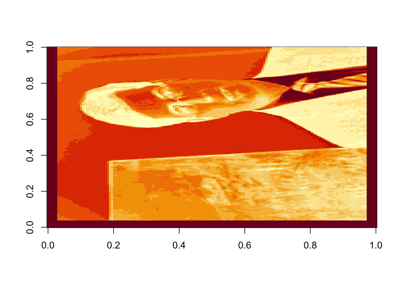
Figure 16.6: Intensity of green in each pixel of the original image
Oops! Dr. Rappa is sideways. To rotate the graphic, we actually have to rotate our coordinate system. There is an easy way to do this (with a little bit of matrix experience), we simply transpose the matrix and then reorder the columns so the last one is first: (note that nrow(rappa.green) gives the number of columns in the transposed matrix)
rappa.green=t(rappa.green)[,nrow(rappa.green):1]
image(rappa.green)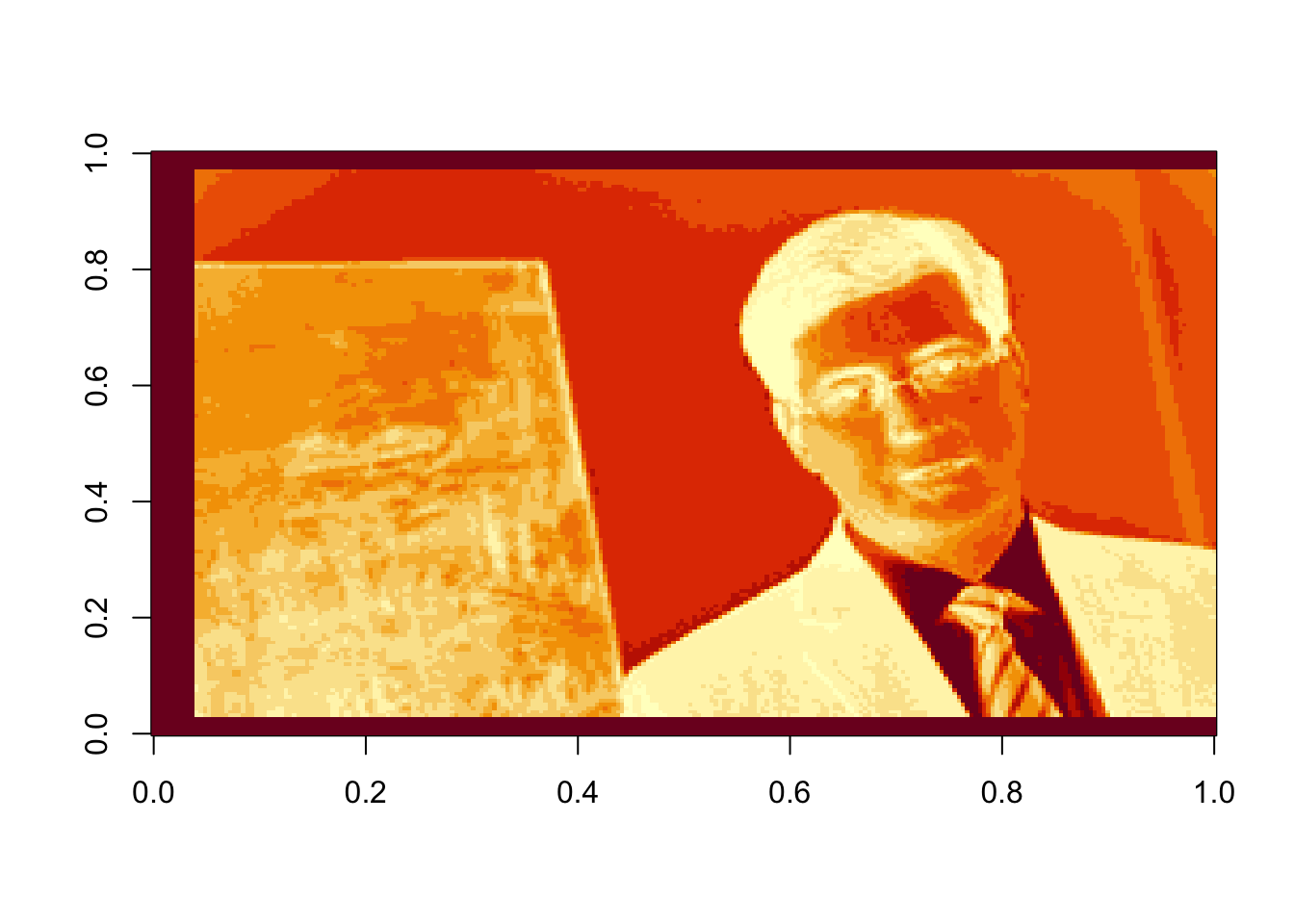
Rather than compressing the colors individually, let’s work with the grayscale image:
greyrappa = read.pnm("LAdata/rappa.pgm")## Warning in rep(cellres, length = 2): 'x' is NULL so the result will be NULLstr(greyrappa)## Formal class 'pixmapGrey' [package "pixmap"] with 6 slots
## ..@ grey : num [1:160, 1:250] 1 1 1 1 1 1 1 1 1 1 ...
## ..@ channels: chr "grey"
## ..@ size : int [1:2] 160 250
## ..@ cellres : num [1:2] 1 1
## ..@ bbox : num [1:4] 0 0 250 160
## ..@ bbcent : logi FALSErappa.grey=greyrappa@grey
#again, rotate 90 degrees
rappa.grey=t(rappa.grey)[,nrow(rappa.grey):1]image(rappa.grey, col=grey((0:1000)/1000))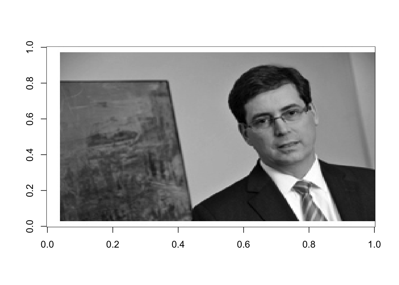
Figure 16.7: Greyscale representation of original image
16.2.2 Computing the SVD of Dr. Rappa
Now, let’s use what we know about the SVD to compress this image. First, let’s compute the SVD and save the individual components. Remember that the rows of \(\mathbf{v}^T\) are the right singular vectors. R outputs the matrix \(\mathbf{v}\) which has the singular vectors in columns.
rappasvd=svd(rappa.grey)
U=rappasvd$u
d=rappasvd$d
Vt=t(rappasvd$v)
Now let’s compute some approximations of rank 3, 10 and 50:
rappaR3=U[ ,1:3]%*%diag(d[1:3])%*%Vt[1:3, ]
image(rappaR3, col=grey((0:1000)/1000))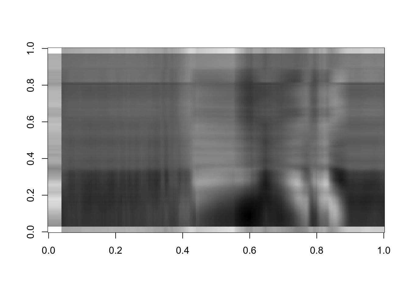
Figure 16.8: Rank 3 approximation of the image data
rappaR10=U[ ,1:10]%*%diag(d[1:10])%*%Vt[1:10, ]
image(rappaR10, col=grey((0:1000)/1000))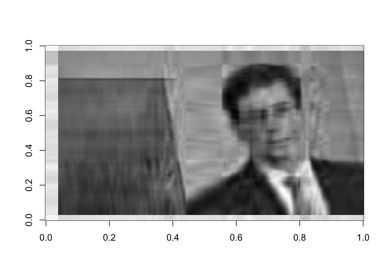
Figure 16.9: Rank 10 approximation of the image data
rappaR25=U[ ,1:25]%*%diag(d[1:25])%*%Vt[1:25, ]
image(rappaR25, col=grey((0:1000)/1000))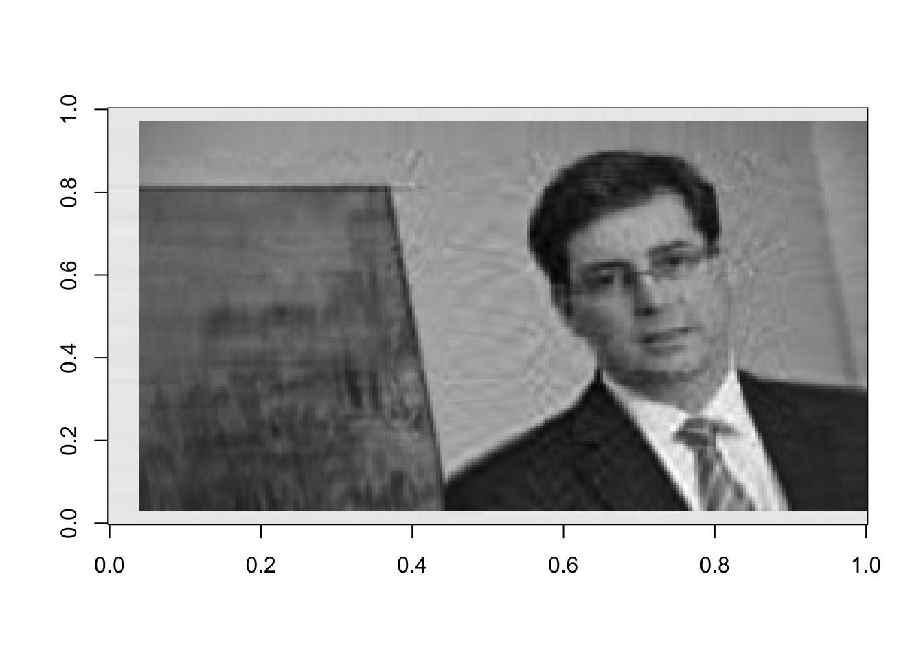
Figure 16.10: Rank 50 approximation of the image data
How many singular vectors does it take to recognize Dr. Rappa? Certainly 25 is sufficient. Can you recognize him with even fewer? You can play around with this and see how the image changes.
16.2.3 The Noise
One of the main benefits of the SVD is that the signal-to-noise ratio of each component decreases as we move towards the right end of the SVD sum. If \(\mathbf{x}\) is our data matrix (in this example, it is a matrix of pixel data to create an image) then,
\[\begin{equation} \mathbf{X}= \sigma_1\mathbf{u}_1\mathbf{v}_1^T + \sigma_2\mathbf{u}_2\mathbf{v}_2^T + \sigma_3\mathbf{u}_3\mathbf{v}_3^T + \dots + \sigma_r\mathbf{u}_r\mathbf{v}_r^T \tag{15.2} \end{equation}\]
where \(r\) is the rank of the matrix. Our image matrix is full rank, \(r=160\). This is the number of nonzero singular values, \(\sigma_i\). But, upon examinination, we see many of the singular values are nearly 0. Let’s examine the last 20 singular values:
d[140:160]## [1] 0.035731961 0.033644986 0.033030189 0.028704912 0.027428124 0.025370919
## [7] 0.024289497 0.022991926 0.020876657 0.020060538 0.018651373 0.018011032
## [13] 0.016299834 0.015668836 0.013928107 0.013046327 0.011403096 0.010763141
## [19] 0.009210187 0.008421977 0.004167310We can think of these values as the amount of “information” directed along those last 20 singular components. If we assume the noise in the image or data is uniformly distributed along each orthogonal component \(\mathbf{u}_i\mathbf{v}_i^T\), then there is just as much noise in the component \(\sigma_1\mathbf{u}_1\mathbf{v}_1^T\) as there is in the component \(\sigma_{160}\mathbf{u}_{160}\mathbf{v}_{160}^T\). But, as we’ve just shown, there is far less information in the component \(\sigma_{160}\mathbf{u}_{160}\mathbf{v}_{160}^T\) than there is in the component \(\sigma_1\mathbf{u}_1\mathbf{v}_1^T\). This means that the later components are primarily noise. Let’s see if we can illustrate this using our image. We’ll construct the parts of the image that are represented on the last few singular components
# Using the last 25 components:

rappa_bad25=U[ ,135:160]%*%diag(d[135:160])%*%Vt[135:160, ]
image(rappa_bad25, col=grey((0:1000)/1000))
Figure 16.11: The last 25 components, or the sum of the last 25 terms in equation (15.2)
# Using the last 50 components:

rappa_bad50=U[ ,110:160]%*%diag(d[110:160])%*%Vt[110:160, ]
image(rappa_bad50, col=grey((0:1000)/1000))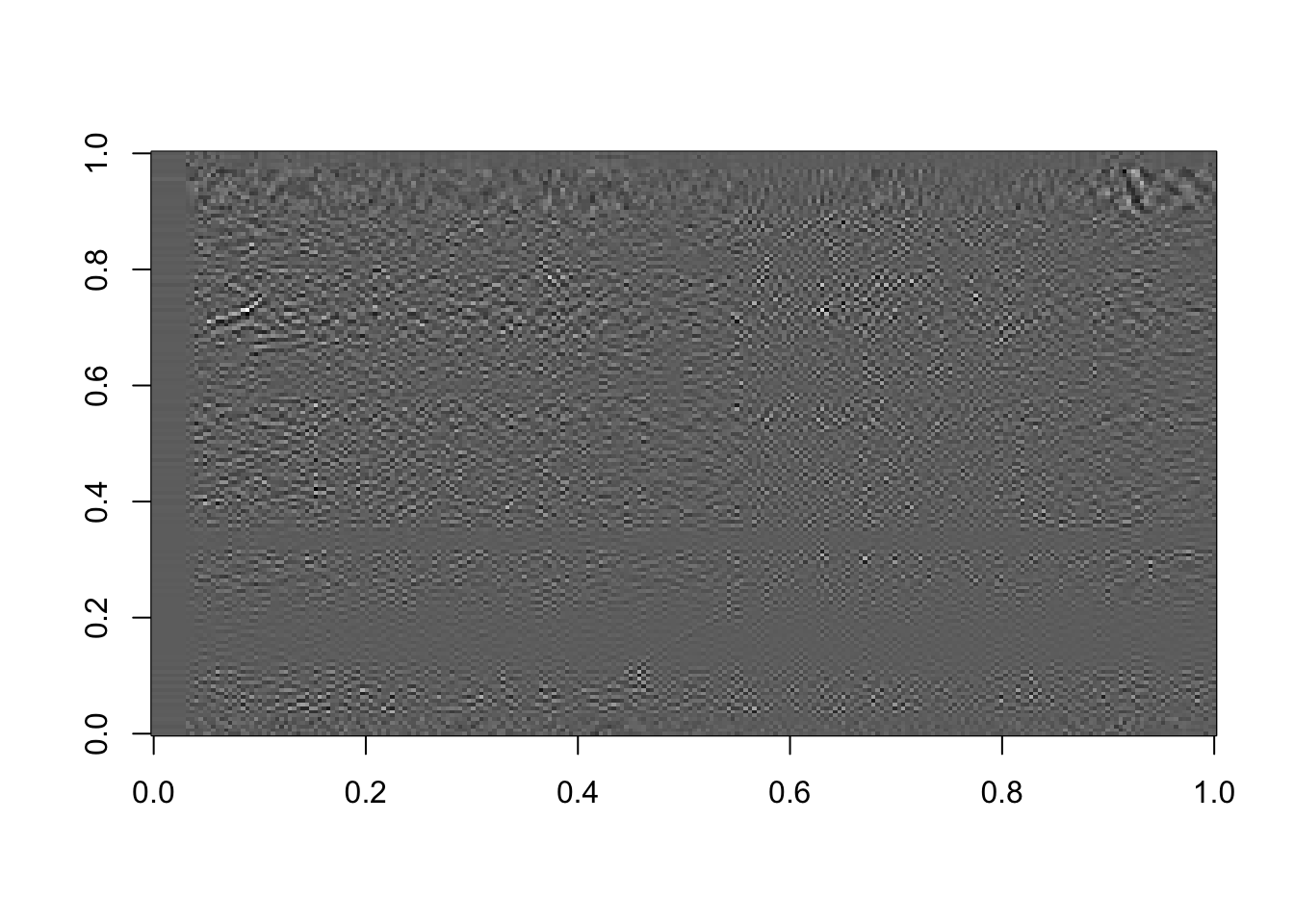
Figure 16.12: The last 50 components, or the sum of the last 50 terms in equation (15.2)
# Using the last 100 components: (4 times as many components as it took us to recognize the face on the front end)

rappa_bad100=U[ ,61:160]%*%diag(d[61:160])%*%Vt[61:160, ]
image(rappa_bad100, col=grey((0:1000)/1000))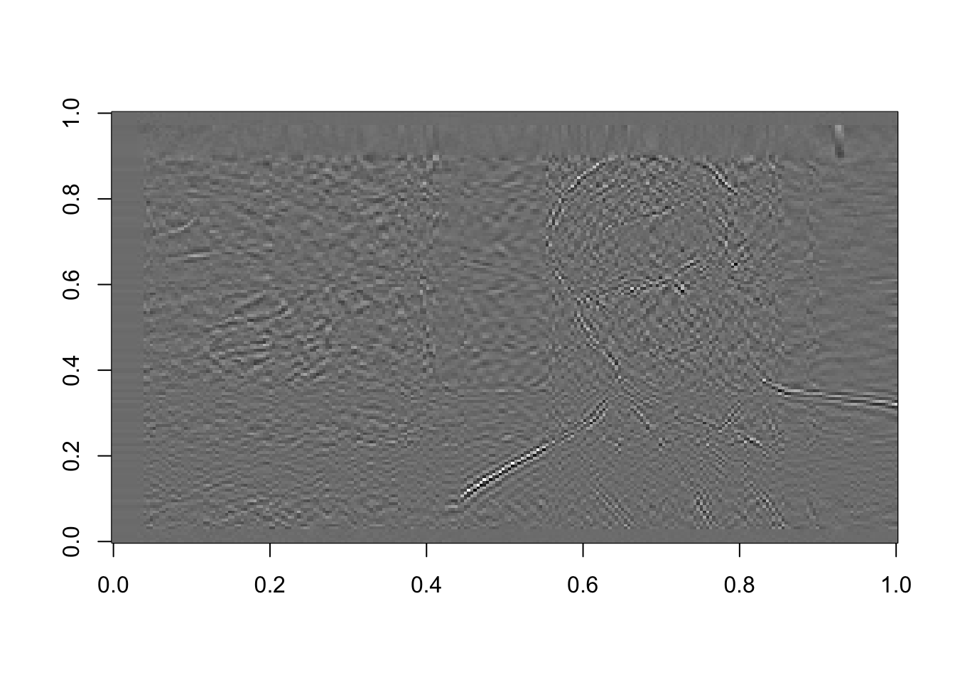
Figure 16.13: The last 100 components, or the sum of the last 100 terms in equation (15.2)
Mostly noise. In the last of these images, we see the outline of Dr. Rappa. One of the first things to go when images are compressed are the crisp outlines of objects. This is something you may have witnessed in your own experience, particularly when changing the format of a picture to one that compresses the size.