Chapter 17 Factor Analysis
Factor Analysis is about looking for underlying relationships or associations. In that way, factor analysis is a correlational study of variables, aiming to group or cluster variables along dimensions. It may also be used to provide an estimate (factor score) of a latent construct which is a linear combination of variables. For example, a standardized test might ask hundreds of questions on a variety of quantitative and verbal subjects. Each of these questions could be viewed as a variable. However, the quantitative questions collectively are meant to measure some latent factor, that is the individual’s quantitative reasoning. A Factor Analysis might be able to reveal these two latent factors (quantitative reasoning and verbal ability) and then also provide an estimate (score) for each individual on each factor.
Any attempt to use factor analysis to summarize or reduce a set to data should be based on a conceptual foundation or hypothesis. It should be remembered that factor analysis will produce factors for most sets of data. Thus, if you simply analyze a large number of variables in the hopes that the technique will “figure it out,” your results may look as though they are grasping at straws. The quality or meaning/interpretation of the derived factors is best when related to a conceptual foundation that existed prior to the analysis.
17.1 Assumptions of Factor Analysis
- No outliers in the data set
-
Adequate sample size
- As a rule of thumb, maintain a ratio of variables to factors of at least 3 (some say 5). This depends on the application.
- You should have at least 10 observations for each variable (some say 20). This often depends on what value of factor loading you want to declare as significant. See Table 17.2 for the details on this.
- No perfect multicollinearity
- Homoskedasticity not required between variables (all variances not required to be equal)
- Linearity of variables desired - only models linear correlation between variables
- Interval data (as opposed to nominal)
- Measurement error on the variables/observations has constant variance and is, on average, 0
- Normality is not required
17.2 Determining Factorability
Before we even begin the process of factor analysis, we have to do some preliminary work to determine whether or not the data even lends itself to this technique. If none of our variables are correlated, then we cannot group them together in any meaningful way! Bartlett’s Sphericity Test and the KMO index are two statistical tests for whether or not a set of variables can be factored. These tests do not provide information about the appropriate number of factors, only whether or not such factors even exist.
17.2.1 Visual Examination of Correlation Matrix
Depending on how many variables you are working with, you may be able to determine whether or not to proceed with factor analysis by simply examining the correlation matrix. With this examination, we are looking for two things:
- Correlations that are significant at the 0.01 level of significance. At least half of the correlations should be significant in order to proceed to the next step.
- Correlations are “sufficient” to justify applying factor analysis. As a rule of thumb, at least half of the correlations should be greater than 0.30.
17.2.2 Barlett’s Sphericity Test
Barlett’s sphericity test checks if the observed correlation matrix is significantly different from the identity matrix. Recall that the correlation of two variables is equal to 0 if and only if they are orthogonal (and thus completely uncorrelated). When this is the case, we cannot reduce the number of variables any further and neither PCA nor any other flavor of factor analysis will be able to compress the information reliably into fewer dimensions. For Barlett’s test, the null hypothesis is: \[H_0 = \mbox{ The variables are orthogonal,} \] which implies that there are no underlying factors to be uncovered. Obviously, we must be able to reject this hypothesis for a meaningful factor model.
17.2.3 Kaiser-Meyer-Olkin (KMO) Measure of Sampling Adequacy
The goal of the Kaiser-Meyer-Olkin (KMO) measure of sampling adequacy is similar to that of Bartlett’s test in that it checks if we can factorize the original variables efficiently. However, the KMO measure is based on the idea of partial correlation [1]. The correlation matrix is always the starting point. We know that the variables are more or less correlated, but the correlation between two variables can be influenced by the others. So, we use the partial correlation in order to measure the relation between two variables by removing the effect of the remaining variables. The KMO index compares the raw values of correlations between variables and those of the partial correlations. If the KMO index is high (\(\approx 1\)), then PCA can act efficiently; if the KMO index is low (\(\approx 0\)), then PCA is not relevant. Generally a KMO index greater than 0.5 is considered acceptable to proceed with factor analysis. Table 17.1 contains the information about interpretting KMO results that was provided in the original 1974 paper.
| KMO value |
Degree of Common Variance |
| 0.90 to 1.00 | Marvelous |
| 0.80 to 0.89 | Middling |
| 0.60 to 0.69 | Mediocre |
| 0.50 to 0.59 | Miserable |
| 0.00 to 0.49 | Don’t Factor |
So, for example, if you have a survey with 100 questions/variables and you obtained a KMO index of 0.61, this tells you that the degree of common variance between your variables is mediocre, on the border of being miserable. While factor analysis may still be appropriate in this case, you will find that such an analysis will not account for a substantial amount of variance in your data. It may still account for enough to draw some meaningful conclusions, however.
17.2.4 Significant factor loadings
When performing principal factor analysis on the correlation matrix, we have some clear guidelines for what kind of factor loadings will be deemed “significant” from a statistical viewpoint based on sample size. Table 17.2 provides those limits.
|
Sample Size Needed for Significance | Factor Loading |
| 350 | .30 |
| 250 | .35 |
| 200 | .40 |
| 150 | .45 |
| 120 | .50 |
| 100 | .55 |
| 85 | .60 |
| 70 | .65 |
| 60 | .70 |
| 50 | .75 |
17.3 Communalities
You can think of communalities as multiple \(R^2\) values for regression models predicting the variables of interest from the factors (the reduced number of factors that your model uses). The communality for a given variable can be interpreted as the proportion of variation in that variable explained by the chosen factors.
Take for example the SAS output for factor analysis on the Iris dataset shown in Figure ??. The factor model (which settles on only one single factor) explains 98% of the variability in petal length. In other words, if you were to use this factor in a simple linear regression model to predict petal length, the associated \(R^2\) value should be 0.98. Indeed you can verify that this is true. The results indicate that this single factor model will do the best job explaining variability in petal length, petal width, and sepal length.
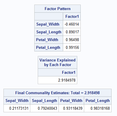
Figure 17.1: SAS output for PROC FACTOR using Iris Dataset
One assessment of how well a factor model is doing can be obtained from the communalities. What you want to see is values that are close to one. This would indicate that the model explains most of the variation for those variables. In this case, the model does better for some variables than it does for others.
If you take all of the communality values, \(c_i\) and add them up you can get a total communality value:
\[\sum_{i=1}^p \widehat{c_i} = \sum_{i=1}^k \widehat{\lambda_i}\]
Here, the total communality is 2.918. The proportion of the total variation explained by the three factors is \[\frac{2.918}{4}\approx 0.75.\] The denominator in that fraction comes from the fact that the correlation matrix is used by default and our dataset has 4 variables. Standardized variables have variance of 1 so the total variance is 4. This gives us the percentage of variation explained in our model. This might be looked at as an overall assessment of the performance of the model. The individual communalities tell how well the model is working for the individual variables, and the total communality gives an overall assessment of performance.
17.4 Number of Factors
A common rule of thumb for determining the number of factors in principal factor analysis on the correlation matrix is to only choose factors with associated eigenvalue (or variance) greater than 1. Since the correlation matrix implies the use of standardized data, each individual variable going in has a variance of 1. So this rule of thumb simply states that we want our factors to explain more variance than any individual variable from our dataset. If this rule of thumb produces too many factors, it is reasonable to raise that limiting condition only if the number of factors still explains a reasonable amount of the total variance.
17.5 Rotation of Factors
The purpose of rotating factors is to make them more interpretable. If factor loadings are relatively constant across variables, they don’t help us find latent structure or clusters of variables. This will often happen in PCA when the goal is only to find directions of maximal variance. Thus, once the number of components/factors is fixed and a projection of the data onto a lower-dimensional subspace is done, we are free to rotate the axes of the result without losing any variance. The axes will no longer be principal components! The amount of variance explained by each factor will change, but the total amount of variance in the reduced data will stay the same because all we have done is rotate the basis. The goal is to rotate the factors in such a way that the loading matrix develops a more sparse structure. A sparse loading matrix (one with lots of very small entries and few large entries) is far easier to interpret in terms of finding latent variable groups.
The two most common rotations are varimax and quartimax. The goal of varimax rotation is to maximize the squared factor loadings in each factor, i.e. to simplify the columns of the factor matrix. In each factor, the large loadings are increased and the small loadings are decreased so that each factor has only a few variables with large loadings. In contrast, the goal of quartimax rotation is to simply the rows of the factor matrix. In each variable the large loadings are increased and the small loadings are decreased so that each variable will only load on a few factors. Which of these factor rotations is appropriate
17.6 Methods of Factor Analysis
Factor Analysis is much like PCA in that it attempts to find some latent variables (linear combinations of original variables) which can describe large portions of the total variance in data. There are numerous ways to compute factors for factor analysis, the two most common methods are:
- The principal axis method (i.e. PCA) and
- Maximum Likelihood Estimation.
In fact, the default method for SAS’s PROC FACTOR with no additional options is merely PCA. For some reason, the scores and factors may be scaled differently, involving the standard deviations of each factor, but nonetheless, there is absolutely nothing different between PROC FACTOR defaults and PROC PRINCOMP.
The difference between Factor Analysis and PCA is two-fold:
- In factor analysis, the factors are usually rotated to obtain a more sparse (i.e. interpretable) structure varimax rotation is the most common rotation. Others include promax, and quartimax.)
- The factors try to only explain the “common variance” between variables. In other words, Factor Analysis tries to estimate how much of each variable’s variance is specific to that variable and not “covarying” (for lack of a better word) with any other variables. This specific variance is often subtracted from the diagonal of the covariance matrix before factors or components are found.
We’ll talk more about the first difference than the second because it generally carries more advantages.
17.6.1 PCA Rotations
Let’s first talk about the motivation behind principal component rotations. Compare the following sets of (fabricated) factors, both using the variables from the iris dataset. Listed below are the loadings of each variable on two factors. Which set of factors is more easily interpretted?
| Variable | P1 | P2 |
| Sepal.Length | -.3 | .7 |
| Sepal.Width | -.5 | .4 |
| Petal.Length | .7 | .3 |
| Petal.Width | .4 | -.5 |
| Variable | F1 | F2 |
| Sepal.Length | 0 | .9 |
| Sepal.Width | -.9 | 0 |
| Petal.Length | .8 | 0 |
| Petal.Width | .1 | -.9 |
The difference between these factors might be described as “sparsity.” Factor Set 2 has more zero loadings than Factor Set 1. It also has entries which are comparitively larger in magnitude. This makes Factor Set 2 much easier to interpret! Clearly F1 is dominated by the variables Sepal.Width (positively correlated) and Petal.Length (negatively correlated), whereas F2 is dominated by the variables Sepal.Length (positively) and Petal.Width (negatively). Factor interpretation doesn’t get much easier than that! With the first set of factors, the story is not so clear.
This is the whole purpose of factor rotation, to increase the interpretability of factors by encouraging sparsity. Geometrically, factor rotation tries to rotate a given set of factors (like those derived from PCA) to be more closely aligned with the original variables once the dimensions of the space have been reduced and the variables have been pushed closer together in the factor space. Let’s take a look at the actual principal components from the iris data and then rotate them using a varimax rotation. In order to rotate the factors, we have to decide on some number of factors to use. If we rotated all 4 orthogonal components to find sparsity, we’d just end up with our original variables again!
irispca = princomp(iris[,1:4],scale=T)## Warning: In princomp.default(iris[, 1:4], scale = T) :
## extra argument 'scale' will be disregardedsummary(irispca)## Importance of components:
## Comp.1 Comp.2 Comp.3 Comp.4
## Standard deviation 2.0494032 0.49097143 0.27872586 0.153870700
## Proportion of Variance 0.9246187 0.05306648 0.01710261 0.005212184
## Cumulative Proportion 0.9246187 0.97768521 0.99478782 1.000000000irispca$loadings##
## Loadings:
## Comp.1 Comp.2 Comp.3 Comp.4
## Sepal.Length 0.361 0.657 0.582 0.315
## Sepal.Width 0.730 -0.598 -0.320
## Petal.Length 0.857 -0.173 -0.480
## Petal.Width 0.358 -0.546 0.754
##
## Comp.1 Comp.2 Comp.3 Comp.4
## SS loadings 1.00 1.00 1.00 1.00
## Proportion Var 0.25 0.25 0.25 0.25
## Cumulative Var 0.25 0.50 0.75 1.00# Since 2 components explain a large proportion of the variation, lets settle on those two:
rotatedpca = varimax(irispca$loadings[,1:2])
rotatedpca$loadings##
## Loadings:
## Comp.1 Comp.2
## Sepal.Length 0.223 0.716
## Sepal.Width -0.229 0.699
## Petal.Length 0.874
## Petal.Width 0.366
##
## Comp.1 Comp.2
## SS loadings 1.00 1.00
## Proportion Var 0.25 0.25
## Cumulative Var 0.25 0.50# Not a drastic amount of difference, but clearly an attempt has been made to encourage
# sparsity in the vectors of loadings.
# NOTE: THE ROTATED FACTORS EXPLAIN THE SAME AMOUNT OF VARIANCE AS THE FIRST TWO PCS
# AFTER PROJECTING THE DATA INTO TWO DIMENSIONS (THE BIPLOT) ALL WE DID WAS ROTATE THOSE
# ORTHOGONAL AXIS. THIS CHANGES THE PROPORTION EXPLAINED BY *EACH* AXIS, BUT NOT THE TOTAL
# AMOUNT EXPLAINED BY THE TWO TOGETHER.
# The output from varimax can't tell you about proportion of variance in the original data
# because you didn't even tell it what the original data was!17.7 Case Study: Personality Tests
In this example, we’ll use a publicly available dataset that describes personality traits of nearly Read in the Big5 Personality test dataset, which contains likert scale responses (five point scale where 1=Disagree, 3=Neutral, 5=Agree. 0 = missing) on 50 different questions in columns 8 through 57. The questions, labeled E1-E10 (E=extroversion), N1-N10 (N=neuroticism), A1-A10 (A=agreeableness), C1-C10 (C=conscientiousness), and O1-O10 (O=openness) all attempt to measure 5 key angles of human personality. The first 7 columns contain demographic information coded as follows:
-
Race Chosen from a drop down menu.
- 1=Mixed Race
- 2=Arctic (Siberian, Eskimo)
- 3=Caucasian (European)
- 4=Caucasian (Indian)
- 5=Caucasian (Middle East)
- 6=Caucasian (North African, Other)
- 7=Indigenous Australian
- 8=Native American
- 9=North East Asian (Mongol, Tibetan, Korean Japanese, etc)
- 10=Pacific (Polynesian, Micronesian, etc)
- 11=South East Asian (Chinese, Thai, Malay, Filipino, etc)
- 12=West African, Bushmen, Ethiopian
- 13=Other (0=missed)
- Age Entered as text (individuals reporting age < 13 were not recorded)
-
Engnat Response to “is English your native language?”
- 1=yes
- 2=no
- 0=missing
-
Gender Chosen from a drop down menu
- 1=Male
- 2=Female
- 3=Other
- 0=missing
-
Hand “What hand do you use to write with?”
- 1=Right
- 2=Left
- 3=Both
- 0=missing
options(digits=2)
big5 = read.csv('http://birch.iaa.ncsu.edu/~slrace/LinearAlgebra2021/Code/big5.csv')
To perform the same analysis we did in SAS, we want to use Correlation PCA and rotate the axes with a varimax transformation. We will start by performing the PCA. We need to set the option scale=T to perform PCA on the correlation matrix rather than the default covariance matrix. We will only compute the first 5 principal components because we have 5 personality traits we are trying to measure. We could also compute more than 5 and take the number of components with eigenvalues >1 to match the default output in SAS (without n=5 option).
17.7.1 Raw PCA Factors
options(digits=5)
pca.out = prcomp(big5[,8:57], rank = 5, scale = T)
Remember the only difference between the default PROC PRINCOMP output and the default PROC FACTOR output in SAS was the fact that the eigenvectors in PROC PRINCOMP were normalized to be unit vectors and the factor vectors in PROC FACTOR were those same eigenvectors scaled by the square roots of the eigenvalues. So we want to multiply each eigenvector column output in pca.out$rotation (recall this is the loading matrix or matrix of eigenvectors) by the square root of the corresponding eigenvalue given in pca.out$sdev. You’ll recall that multiplying a matrix by a diagonal matrix on the right has the effect of scaling the columns of the matrix. So we’ll just make a diagonal matrix, \(\textbf{S}\) with diagonal elements from the pca.out$sdev vector and scale the columns of the pca.out$rotation matrix. Similarly, the coordinates of the data along each component then need to be divided by the standard deviation to cancel out this effect of lengthening the axis. So again we will multiply by a diagonal matrix to perform this scaling, but this time, we use the diagonal matrix \(\textbf{S}^{-1}=\) diag(1/(pca.out$sdev)).
Matrix multiplication in R is performed with the \%\*\% operator.
fact.loadings = pca.out$rotation[,1:5] %*% diag(pca.out$sdev[1:5])
fact.scores = pca.out$x[,1:5] %*%diag(1/pca.out$sdev[1:5])
# PRINT OUT THE FIRST 5 ROWS OF EACH MATRIX FOR CONFIRMATION.
fact.loadings[1:5,1:5]
## [,1] [,2] [,3] [,4] [,5]
## E1 -0.52057 0.27735 -0.29183 0.13456 -0.25072
## E2 0.51025 -0.35942 0.26959 -0.14223 0.21649
## E3 -0.70998 0.15791 -0.11623 0.21768 -0.11303
## E4 0.58361 -0.20341 0.31433 -0.17833 0.22788
## E5 -0.65751 0.31924 -0.16404 0.12496 -0.21810fact.scores[1:5,1:5]## [,1] [,2] [,3] [,4] [,5]
## [1,] -2.53286 -1.16617 0.276244 0.043229 -0.069518
## [2,] 0.70216 -1.22761 1.095383 1.615919 -0.562371
## [3,] -0.12575 1.33180 1.525208 -1.163062 -2.949501
## [4,] 1.29926 1.17736 0.044168 -0.784411 0.148903
## [5,] -0.37359 0.47716 0.292680 1.233652 0.406582This should match the output from SAS and it does. Remember these columns are unique up to a sign, so you’ll see factor 4 does not have the same sign in both software outputs. This is not cause for concern.
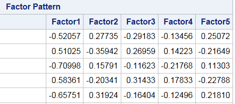
Figure 17.2: Default (Unrotated) Factor Loadings Output by SAS
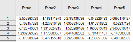
Figure 17.3: Default (Unrotated) Factor Scores Output by SAS
17.7.2 Rotated Principal Components
The next task we may want to undertake is a rotation of the factor axes according to the varimax procedure. The most simple way to go about this is to use the varimax() function to find the optimal rotation of the eigenvectors in the matrix pca.out$rotation. The varimax() function outputs both the new set of axes in the matrix called loadings and the rotation matrix (rotmat) which performs the rotation from the original principal component axes to the new axes. (i.e. if \(\textbf{V}\) contains the old axes as columns and \(\hat{\textbf{V}}\) contains the new axes and \(\textbf{R}\) is the rotation matrix then \(\hat{\textbf{V}} = \textbf{V}\textbf{R}\).) That rotation matrix can be used to perform the same rotation on the scores of the observations. If the matrix \(\textbf{U}\) contains the scores for each observation, then the rotated scores \(\hat{\textbf{U}}\) are found by \(\hat{\textbf{U}} = \textbf{U}\textbf{R}\)
varimax.out = varimax(fact.loadings)
rotated.fact.loadings = fact.loadings %*% varimax.out$rotmat
rotated.fact.scores = fact.scores %*% varimax.out$rotmat
# PRINT OUT THE FIRST 5 ROWS OF EACH MATRIX FOR CONFIRMATION.
rotated.fact.loadings[1:5,]
## [,1] [,2] [,3] [,4] [,5]
## E1 -0.71232 -0.0489043 0.010596 -0.03206926 0.055858
## E2 0.71592 -0.0031185 0.028946 0.03504236 -0.121241
## E3 -0.66912 -0.2604049 0.131609 0.01704690 0.263679
## E4 0.73332 0.1528552 -0.023367 0.00094685 -0.053219
## E5 -0.74534 -0.0757539 0.100875 -0.07140722 0.218602rotated.fact.scores[1:5,]## [,1] [,2] [,3] [,4] [,5]
## [1,] -1.09083 -2.04516 1.40699 -0.38254 0.5998386
## [2,] 0.85718 -0.19268 1.07708 2.03665 -0.2178616
## [3,] -0.92344 2.58761 2.43566 -0.80840 -0.1833138
## [4,] 0.61935 1.53087 -0.79225 -0.59901 -0.0064665
## [5,] -0.39495 -0.10893 -0.24892 0.99744 0.9567712And again we can see that these line up with our SAS Rotated output, however the order does not have to be the same! SAS conveniently reorders the columns according to the variance of the data along that new direction. Since we have not done that in R, the order of the columns is not the same! Factors 1 and 2 are the same in both outputs, but SAS Factor 3 = R Factor 4 and SAS Factor 5 = (-1)* R Factor 4. The coordinates are switched too so nothing changes in our interpretation. Remember, when you rotate factors, you no longer keep the notion that the “first vector” explains the most variance unless you reorder them so that is true (like SAS does).
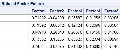
Figure 17.4: Rotated Factor Loadings Output by SAS
knitr::include_graphics('RotatedScores.png')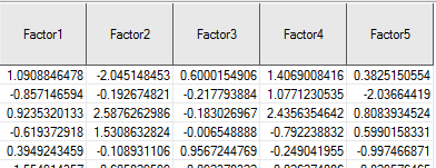
Figure 17.5: Rotated Factor Scores Output by SAS
17.7.3 Visualizing Rotation via BiPlots
Let’s start with a peek at BiPlots of the first 2 of principal component loadings, prior to rotation. Notice that here I’m not going to bother with any scaling of the factor loadings as I’m not interested in forcing my output to look like SAS’s output. I’m also downsampling the observations because 20,000 is far to many to plot.
biplot(pca.out$x[sample(1:19719,1000),1:2],
       pca.out$rotation[,1:2],
       cex=c(0.2,1))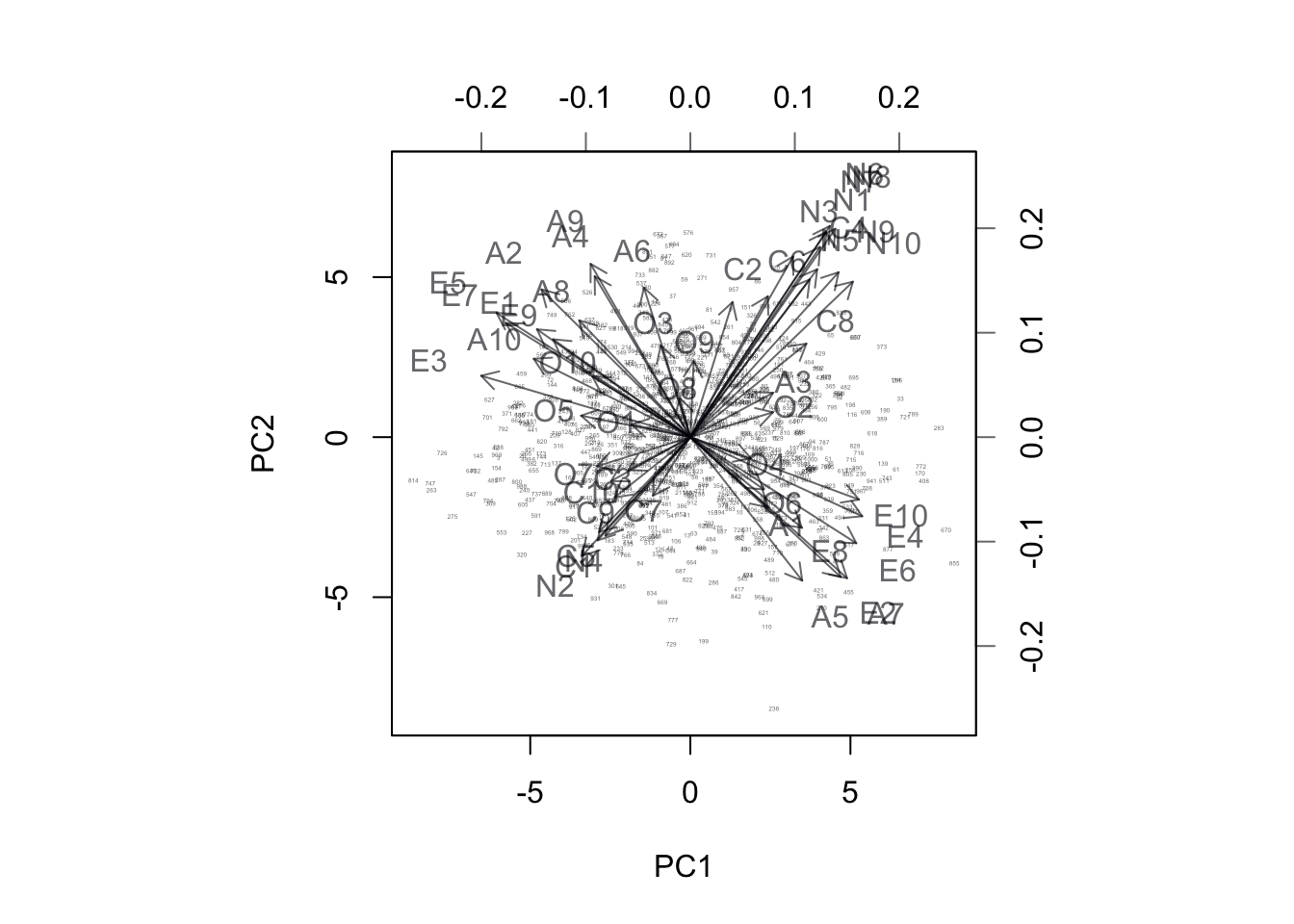
Figure 17.6: BiPlot of Projection onto PC1 and PC2
biplot(pca.out$x[sample(1:19719,1000),3:4],
       pca.out$rotation[,3:4],
       cex=c(0.2,1))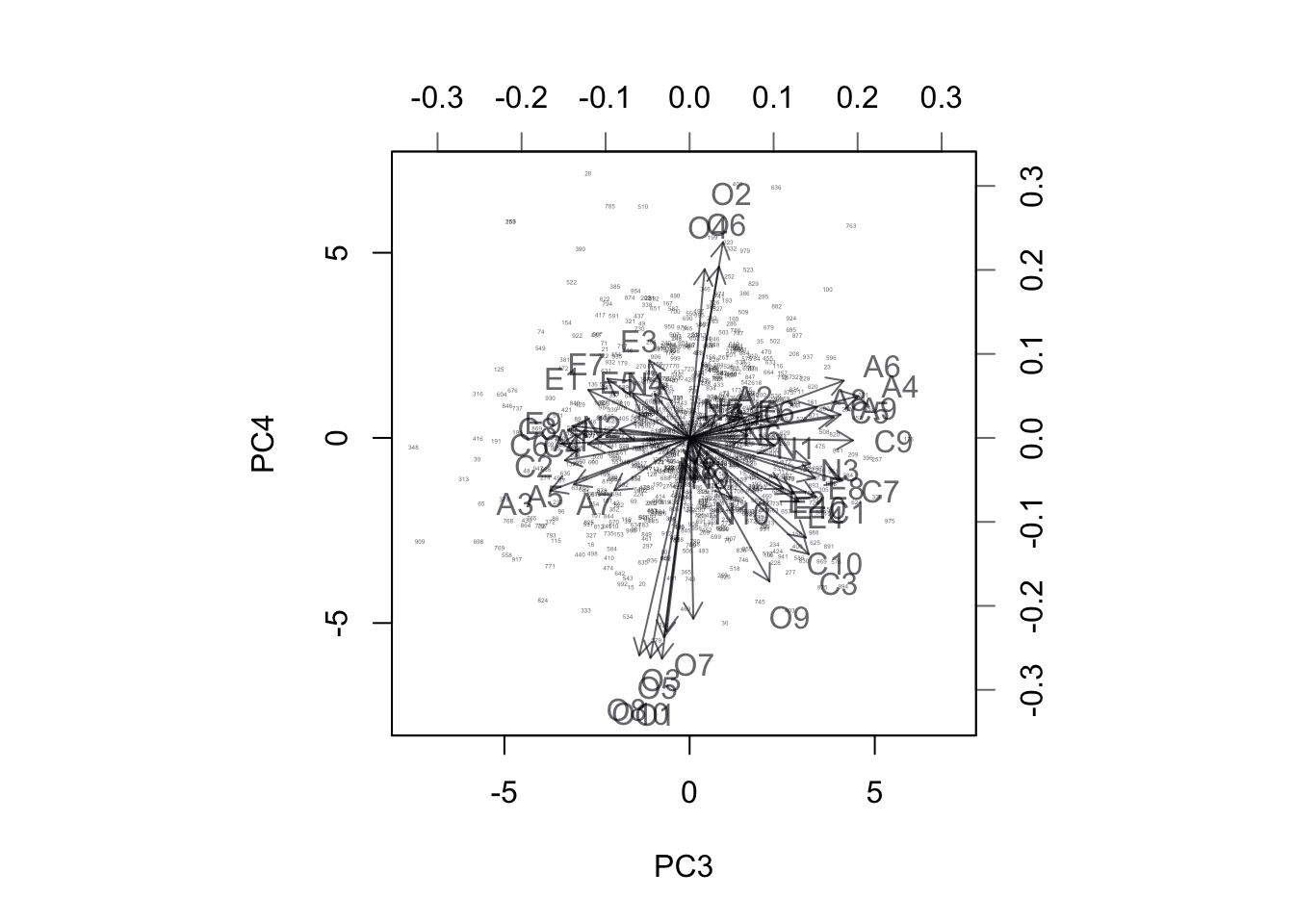
Figure 17.7: BiPlot of Projection onto PC3 and PC4
Let’s see what happens to these biplots after rotation:
vmax = varimax(pca.out$rotation)
newscores = pca.out$x%*%vmax$rotmat
biplot(newscores[sample(1:19719,1000),1:2],
       vmax$loadings[,1:2],
       cex=c(0.2,1),
       xlab = 'Rotated Axis 1',
       ylab = 'Rotated Axis 2')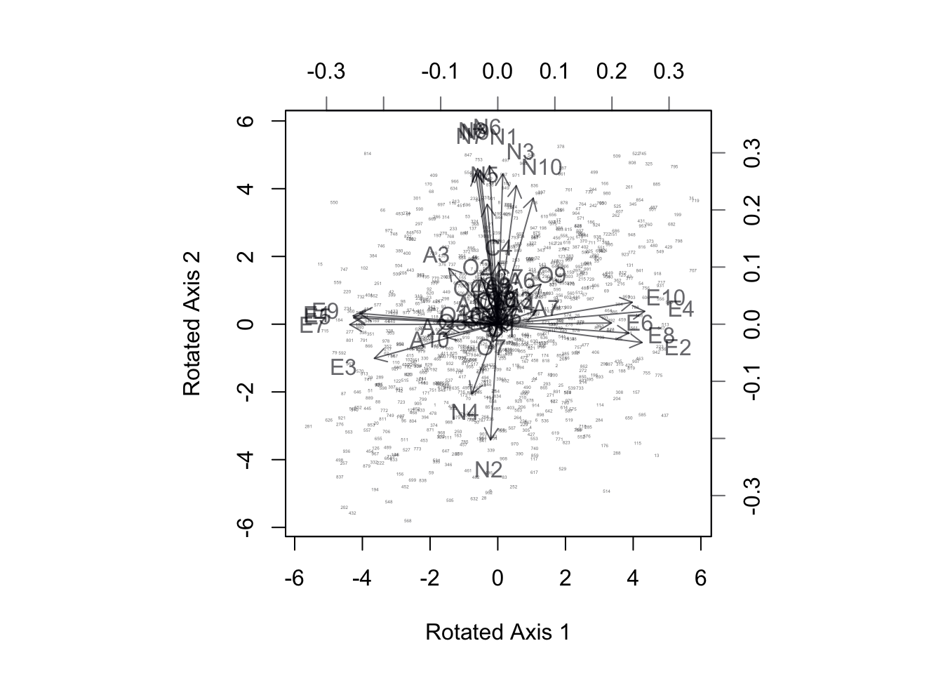
Figure 17.8: BiPlot of Projection onto Rotated Axes 1,2. Extroversion questions align with axis 1, Neuroticism with Axis 2
biplot(newscores[sample(1:19719,1000),3:4],
       vmax$loadings[,3:4],
       cex=c(0.2,1),
       xlab = 'Rotated Axis 3',
       ylab = 'Rotated Axis 4')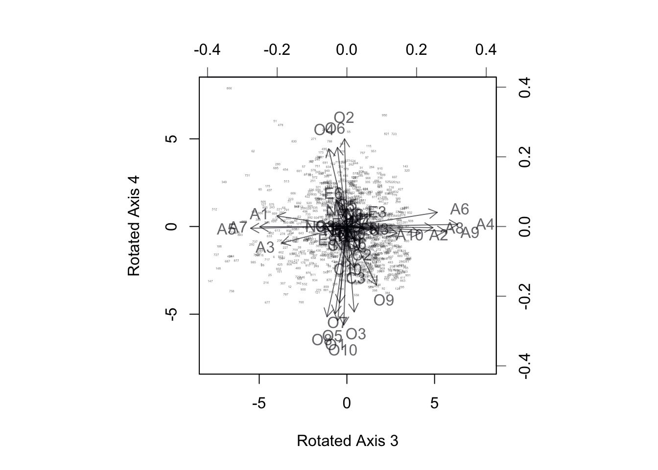
Figure 17.9: BiPlot of Projection onto Rotated Axes 3,4. Agreeableness questions align with axis 3, Openness with Axis 4.
After the rotation, we can see the BiPlots tell a more distinct story. The extroversion questions line up along rotated axes 1, neuroticism along rotated axes 2, and agreeableness and openness are reflected in rotated axes 3 and 4 respectively. The fifth rotated component can be confirmed to represent the last remaining category which is conscientiousness.