Chapter 9 Orthogonality

Orthogonal (or perpendicular) vectors have an angle between them of \(90^{\circ}\), meaning that their cosine (and subsequently their inner product) is zero.

Definition 9.1 (Orthogonality) Two vectors, \(\x\) and \(\y\), are orthogonal in \(n\)-space if their inner product is zero: \[\x^T\y=0\]

Combining the notion of orthogonality and unit vectors we can define an orthonormal set of vectors, or an orthonormal matrix. Remember, for a unit vector, \(\x^T\x = 1\).

Definition 9.2 (Orthonormal Set) The \(n\times 1\) vectors \(\{\x_1,\x_2,\x_3,\dots,\x_p\}\) form an orthonormal set if and only if

\(\x_i^T\x_j = 0\,\) when \(i \ne j\) and
\(\x_i^T\x_i = 1\,\) (equivalently \(\|\mathbf{x}_i\|=1\))

In other words, an orthonormal set is a collection of unit vectors which are mutually orthogonal.

If we form a matrix, \(\X=(\x_1|\x_2|\x_3|\dots|\x_p )\), having an orthonormal set of vectors as columns, we will find that multiplying the matrix by its transpose provides a nice result:

\[\begin{eqnarray*} \X^T\X = \pm \x_1^T \\ \x_2^T \\ \x_3^T \\ \vdots \\ \x_p^T \mp \pm \x_1&\x_2&\x_3&\dots&\x_p \mp &=& \pm \x_1^T\x_1 & \x_1^T\x_2 & \x_1^T\x_3 & \dots & \x_1^T\x_p \\ \x_2^T\x_1 & \x_2^T\x_2 & \x_2^T\x_3 & \dots & \x_2^T\x_p \\ \x_3^T\x_1 & \x_3^T\x_2 & \x_3^T\x_3 &\dots & \x_3^T\x_p \\ \vdots & \vdots & \ddots & \ddots & \vdots \\ \x_p^T\x_1 & \dots & \dots & \ddots & \x_p^T\x_p \mp \\ &=& \pm 1 & 0 & 0 & \dots & 0\\ 0 & 1 & 0 & \dots & 0 \\ 0 & 0 & 1 & \dots & 0 \\ \vdots & \vdots & \ddots & \ddots & \vdots \\ 0 & 0 & 0 & \dots & 1 \mp = \bo{I}_p \end{eqnarray*}\] We will be particularly interested in these types of matrices when they are square. If \(\X\) is a square matrix with orthonormal columns, the arithmetic above means that the inverse of \(\X\) is \(\X^T\) (i.e. \(\X\) also has orthonormal rows): \[\X^T\X=\X\X^T = I.\] Square matrices with orthonormal columns are called orthogonal matrices - this an unfortunate naming mismatch, we agree.

Definition 9.3 (Orthogonal Matrix) A square matrix, \(\bo{U}\) with orthonormal columns also has orthonormal rows and is called an orthogonal matrix. Such a matrix has an inverse which is equal to it’s transpose, \[\U^T\U=\U\U^T = \bo{I} \]

9.1 Orthonormal Basis

Our primary interest in orthonormal sets will be in the formulation of new bases for our data. An orthonormal basis has two advantages over other types of bases, with one advantage stemming from each of the two criteria for orthonormality:

The basis vectors are mutually perpendicular. They are just rotations of the elementary basis vectors and thus when we examine our data in these new bases, we are merely observing a rotation of our data. This allows us to plot the new coordinates of our data on a plane without much regard for the basis vectors themselves. Basis vectors that are not orthogonal would create a distorted image of our data if we did this. We’d need to factor in the angle between the basis vectors to grasp our previously intuitive notions of distance and similarity.
The basis vectors have length 1. So when we look at the coordinates associated with each basis vector, they tell us how many units to go in each direction. This way, again, we can ignore the basis vectors and focus on the coordinates alone. We truly just rotated the axes.

These two advantages combine to mean that we can use our new coordinates in place of our original data without any loss of “signal.” We can rotate my multidimensional data cloud, put that rotated data into a regression or clustering model, and then draw conclusions that about my original data points (of course our “variables” (basis vectors) are no longer the same so we wouldn’t be able to draw any conclusions about our original variables from my regression analysis until we un-rotated the data, but the predictions would all match exactly).

However, the real power of these advantages are the ease with which we can perform orthogonal projections and the ease with which we can transform from our original space to the new space and back again.

9.2 Orthogonal Projection

Think about taking a giant flashlight and shining all of the data onto a subspace at a right angle. The resulting shadow would be the orthogonal projection of the data onto the subspace. Figure 9.1 brings this definition to life.

Figure 9.1: Omitting a variable from an orthonormal basis amounts to orthogonal projection onto the span of the other basis vectors.

Of course, data can exist below and all around the subspace in question, so it might be helpful to imagine two flashlights or many flashlights that project each data point down to the closest point on the subspace (an orthogonal projection onto a subspace of interest always gets you as close to your original data as possible, under the constraint that the projection be contained in the subspace).

When we have a cloud of data and we “drop” one of our variables, geometrically this amounts to an orthogonal projection of the data onto the span of the other axes - reducing the dimensionality of the space in which it exists by 1. Figure 9.2 strives to make this clear.

Figure 9.2: Omitting a variable from an orthonormal basis amounts to orthogonal projection onto the span of the other basis vectors.

9.3 Why??

My favorite question. “Whyyy do we have to learn this?!” It’s time to build some intuition toward that question. Consider the following 3-D scatter plot, which is interactive. Turn it around with your mouse and see what you notice.

Figure 9.3: 3-Dimensional data cloud that suffers from severe multicollinearity.

Does it look like this data is 3-dimensional in nature? It appears that it could be well-summarized if it existed on a plane. However, what is that plane? We can’t merely drop a variable in this instance, as doing so is quite likely to destroy a good proportion of the information from the data. Still, it seems clear that by rotating the data to the right set of axes, we could then squish it down and use 2 coordinates to describe the data without losing much of the information at all. What do we mean by “information?” In this context, using the word “variance” works well. We want to keep as much of the original variance as possible when we squish the cloud down to a plane with an orthogonal projection. Can you find the (approximate) rotation that gives you the best view of the data points?

Figure 9.3 is really the jumping off point. Once we can intuitively see why we might benefit from a new basis and how one might be crafted, we’re ready to start digging in to PCA. Once we’ve exposed the basic terminology in Chapters 12 and 13, we can explore the magnificent world of dimension reduction and its many benefits in the case studies in Chapters 14-18.

9.4 Exercises

Let \[\U=\frac{1}{3}\pm -1&2&0&-2\\2&2&0&1\\0&0&3&0\\-2&1&0&2\mp\]
1. Show that \(\U\) is an orthogonal matrix.
2. Let \(\bo{b}=\pm 1\\1\\1\\1\mp\). Solve the equation \(\U\x=\bo{b}\).
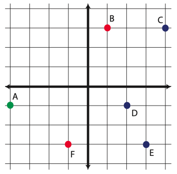
Draw the orthogonal projection of the points onto the subspace \(span \left\lbrace \pm 1\\-1\mp \right\rbrace\)
Are the vectors \(\v_1=\pm 1\\-1\\1 \mp\) and \(\v_2=\pm 0\\1\\1 \mp\) orthogonal? How do you know?
What are the two conditions necessary for a collection of vectors to be orthonormal?
Show that the vectors \(\v_1 = \pm 3 \\ 1\mp\) and \(\v_2=\pm -2 \\6\mp\) are orthogonal. Create an orthonormal basis for \(\Re^2\) using these two direction vectors.
Consider \(\a_1=(1,1)\) and \(\a_2=(0,1)\) as coordinates for points in the elementary basis. Write the coordinates of \(\a_1\) and \(\a_2\) in the orthonormal basis found in the previous exercise. Draw a picture which reflects the old and new basis vectors.
Briefly explain why an orthonormal basis is important.
Find two vectors which are orthogonal to \(\x=\pm 1\\1\\1\mp\)
Pythagorean Theorem. Show that \(\x\) and \(\y\) are orthogonal if and only if \[\|\x+\y\|_2^2 = \|\x\|_2^2 + \|\y\|_2^2\] (Hint: Recall that \(\|\x\|_2^2 = \x^T\x\))