Chapter 12 Eigenvalues and Eigenvectors

Eigenvalues and eigenvectors are (scalar, vector)-pairs that form the “essence” of a matrix. The prefix eigen- is adopted from the German word eigen which means “characteristic, inherent, own” and was introduced by David Hilbert in 1904, but the study of these characteristic directions and magnitudes dates back to Euler’s study of the rotational motion of rigid bodies in the \(18^{th}\) century.

Definition 12.1 (Eigenvalues and Eigenvectors) For a square matrix \(\A_{n\times n}\), a scalar \(\lambda\) is called an eigenvalue of \(\A\) if there is a nonzero vector \(\x\) such that \[\A\x=\lambda\x.\] Such a vector, \(\x\) is called an eigenvector of \(\A\) corresponding to the eigenvalue \(\lambda\). We sometimes refer to the pair \((\lambda,\x)\) as an eigenpair.

Eigenvalues and eigenvectors have numerous applications from graphic design to quantum mechanics to geology to epidemiology. The main application of note for data scientists is Principal Component Analysis, but we will also see eigenvalue equations used in social network analysis to determine important players in a network and to detect communities in the network. Before we dive into those applications, let’s first get a handle on the definition by exploring some examples.

Example 12.1 (Eigenvalues and Eigenvectors) Determine whether \(\x=\pm 1\\1 \mp\) is an eigenvector of \(\A=\pm 3 & 1 \\1&3 \mp\) and if so, find the corresponding eigenvalue.\ To determine whether \(\x\) is an eigenvector, we want to compute \(\A\x\) and observe whether the result is a multiple of \(\x\). If this is the case, then the multiplication factor is the corresponding eigenvalue: \[\A\x=\pm 3 & 1 \\1&3 \mp \pm 1\\1 \mp =\pm 4\\4 \mp=4\pm 1\\1 \mp\] From this it follows that \(\x\) is an eigenvector of \(\A\) and the corresponding eigenvalue is \(\lambda = 4\).\

Is the vector \(\y=\pm 2\\2 \mp\) an eigenvector? \[\A\y=\pm 3 & 1 \\1&3 \mp \pm 2\\2 \mp =\pm 8\\8 \mp=4\pm 2\\2 \mp = 4\y\] Yes, it is and it corresponds to the same eigenvalue, \(\lambda=4\)

Example 12.1 shows a very important property of eigenvalue-eigenvector pairs. If \((\lambda,\x)\) is an eigenpair then any scalar multiple of \(\x\) is also an eigenvector corresponding to \(\lambda\). To see this, let \((\lambda,\x)\) be an eigenpair for a matrix \(\A\) (which means that \(\A\x=\lambda\x\)) and let \(\y=\alpha\x\) be any scalar multiple of \(\x\). Then we have, \[\A\y = \A(\alpha\x)=\alpha(\A\x) = \alpha(\lambda\x) = \lambda(\alpha\x)=\lambda\y\] which shows that \(\y\) (or any scalar multiple of \(\x\)) is also an eigenvector associated with the eigenvalue \(\lambda\).

Thus, for each eigenvalue we have infinitely many eigenvectors. In the preceding example, the eigenvectors associated with \(\lambda = 4\) will be scalar multiples of \(\x=\pm 1\\1 \mp\). You may recall from Chapter 7 that the set of all scalar multiples of \(\x\) is denoted \(span(\x)\). The \(span(\x)\) in this example represents the eigenspace of \(\lambda\). Note: when using software to compute eigenvectors, it is standard practice for the software to provide the normalized/unit eigenvector.

In some situations, an eigenvalue can have multiple eigenvectors which are linearly independent. The number of linearly independent eigenvectors associated with an eigenvalue is called the geometric multiplicity of the eigenvalue. Example 12.2 clarifies this concept.

Example 12.2 (Geometric Multiplicity) Consider the matrix \(\A=\pm 3 & 0 \\0 & 3 \mp\). It should be straightforward to see that \(\x_1 =\pm 1 \\0 \mp\) and \(\x_2=\pm 0\\1\mp\) are both eigenvectors corresponding to the eigenvalue \(\lambda = 3\). \(\x_1\) and \(\x_2\) are linearly independent, therefore the geometric multiplicity of \(\lambda=3\) is 2.

What happens if we take a linear combination of \(\x_1\) and \(\x_2\)? Is that also an eigenvector? Consider \(\y=\pm 2 \\ 3 \mp = 2\x_1+3\x_2\). Then \[\A\y = \pm 3 & 0 \\0 & 3 \mp \pm 2 \\ 3 \mp = \pm 6 \\ 9 \mp = 3 \pm 2\\3\mp = 3\y\] shows that \(\y\) is also an eigenvector associated with \(\lambda=3\).

The eigenspace corresponding to \(\lambda=3\) is the set of all linear combinations of \(\x_1\) and \(\x_2\), i.e. the \(span(\x_1,\x_2)\).

We can generalize the result that we saw in Example 12.2 for any square matrix and any geometric multiplicity. Let \(\A_{n\times n}\) have an eigenvalue \(\lambda\) with geometric multiplicity \(k\). This means there are \(k\) linearly independent eigenvectors, \(\x_1,\x_2,\dots,\x_k\) such that \(\A\x_i=\lambda\x_i\) for each eigenvector \(\x_i\). Now if we let \(\y\) be a vector in the \(span(\x_1,\x_2,\dots,\x_k)\) then \(\y\) is some linear combination of the \(\x_i\)’s: \[\y=\alpha_1\x_2+\alpha_2\x_2+\dots+\alpha_k\x_k\] Observe what happens when we multiply \(\y\) by \(\A\): \[\begin{eqnarray*} \A\y &=&\A(\alpha_1\x_2+\alpha_2\x_2+\dots+\alpha_k\x_k) \\ &=& \alpha_1(\A\x_1)+\alpha_2(\A\x_2)+\dots +\alpha_k(\A\x_k) \\ &=& \alpha_1(\lambda\x_1)+\alpha_2(\lambda\x_2)+\dots +\alpha_k(\lambda\x_k) \\ &=& \lambda(\alpha_1\x_2+\alpha_2\x_2+\dots+\alpha_k\x_k) \\ &=& \lambda\y \end{eqnarray*}\] which shows that \(\y\) (or any vector in the \(span(\x_1,\x_2,\dots,\x_k)\)) is an eigenvector of \(\A\) corresponding to \(\lambda\).

This proof allows us to formally define the concept of an eigenspace.

Definition 12.2 (Eigenspace) Let \(\A\) be a square matrix and let \(\lambda\) be an eigenvalue of \(\A\). The set of all eigenvectors corresponding to \(\lambda\), together with the zero vector, is called the eigenspace of \(\lambda\). The number of basis vectors required to form the eigenspace is called the geometric multiplicity of \(\lambda\).

Now, let’s attempt the eigenvalue problem from the other side. Given an eigenvalue, we will find the corresponding eigenspace in Example 12.3.

Example 12.3 (Eigenvalues and Eigenvectors) Show that \(\lambda=5\) is an eigenvalue of \(\A=\pm 1 & 2 \\4&3 \mp\) and determine the eigenspace of \(\lambda=5\).

Attempting the problem from this angle requires slightly more work. We want to find a vector \(\x\) such that \(\A\x=5\x\). Setting this up, we have: \[\A\x = 5\x.\] What we want to do is move both terms to one side and factor out the vector \(x\). In order to do this, we must use an identity matrix, otherwise the equation wouldn’t make sense (we’d be subtracting a constant from a matrix). \[\begin{eqnarray*} \A\x-5\x &=& \bo{0}\\ (\A-5\bo{I})\x &=& \bo{0} \\ \left( \pm 1 & 2 \\4&3 \mp - \pm 5 & 0 \\ 0 & 5 \mp \right) \pm x_1 \\ x_2 \mp &=& \pm 0 \\0 \mp \\ \pm -4 & 2\\ 4 & -2 \mp \pm x_1 \\ x_2 \mp &=& \pm 0 \\0 \mp \\ \end{eqnarray*}\] Clearly, the matrix \(\A-\lambda\bo{I}\) is singular (i.e. does not have linearly independent rows/columns). This will always be the case by the definition \(\A\x=\lambda\x\), and is often used as an alternative definition.\ In order to solve this homogeneous system of equations, we use Gaussian elimination: \[\left(\begin{array}{rr|r} -4 & 2 & 0 \\4 & -2 & 0 \end{array}\right)\longrightarrow\left(\begin{array}{rr|r} 1 & -\frac{1}{2} & 0 \\0 & 0 & 0 \end{array}\right)\] This implies that any vector \(\x\) for which \(x_1-\frac{1}{2}\x_2=0\) satisfies the eigenvector equation. We can pick any such vector, for example \(\x=\pm 1\\2\mp\), and say that the eigenspace of \(\lambda=5\) is \[span\left\lbrace\pm 1\\2 \mp\right\rbrace\]

If we didn’t know either an eigenvalue or eigenvector of \(\A\) and instead wanted to find both, we would first find eigenvalues by determining all possible \(\lambda\) such that \(\A-\lambda\bo{I}\) is singular and then find the associated eigenvectors. There are some tricks which allow us to do this by hand for \(2\times 2\) and \(3\times 3\) matrices, but after that the computation time is unworthy of the effort. Now that we have a good understanding of how to interpret eigenvalues and eigenvectors algebraically, let’s take a look at some of the things that they can do, starting with one important fact.

Definition 12.3 (Eigenvalues and the Trace of a Matrix) Let \(\A\) be an \(n\times n\) matrix with eigenvalues \(\lambda_1,\lambda_2,\dots,\lambda_n\). Then the sum of the eigenvalues is equal to the trace of the matrix (recall that the trace of a matrix is the sum of its diagonal elements). \[Trace(\A)=\sum_{i=1}^n \lambda_i.\]

Example 12.4 (Trace of Covariance Matrix) Suppose that we had a collection of \(n\) observations on \(p\) variables, \(\x_1,\x_2,\dots,\x_p\). After centering the data to have zero mean, we can compute the sample variances as: \[var(\x_i)=\frac{1}{n-1}\x_i^T\x_i =\|\x_i\|^2\] These variances form the diagonal elements of the sample covariance matrix, \[\ssigma = \frac{1}{n-1}\X^T\X\] Thus, the total variance of this data is \[\frac{1}{n-1}\sum_{i=1}^n \|\x_i\|^2 = Trace(\ssigma) = \sum_{i=1}^n \lambda_i.\]

In other words, the sum of the eigenvalues of a covariance matrix provides the total variance in the variables \(\x_1,\dots,\x_p\).

12.1 Diagonalization

Let’s take another look at Example 12.3. We already showed that \(\lambda_1=5\) and \(\v_1=\pm 1\\2\mp\) is an eigenpair for the matrix \(\A=\pm 1 & 2 \\4&3 \mp\). You may verify that \(\lambda_2=-1\) and \(\v_2=\pm 1\\-1 \mp\) is another eigenpair. Suppose we create a matrix of eigenvectors: \[\V=(\v_1,\v_2) = \pm 1&1\\2&-1 \mp\] and a diagonal matrix containing the corresponding eigenvalues: \[\D=\pm 5 & 0 \\ 0 & -1 \mp\] Then it is easy to verify that \(\A\V=\V\D\): \[\begin{eqnarray*} \A\V &=& \pm 1 & 2 \\4&3 \mp \pm 1&1\\2&-1 \mp\\ &=& \pm 5&-1\\10&1 \mp\\ &=& \pm 1&1\\2&-1 \mp\pm 5 & 0 \\ 0 & -1 \mp\\ &=&\V\D \end{eqnarray*}\] If the columns of \(\V\) are linearly independent, which they are in this case, we can write: \[\V^{-1}\A\V = \D\]

What we have just done is develop a way to transform a matrix \(\A\) into a diagonal matrix \(\D\). This is known as diagonalization.

Definition 12.4 (Diagonalizable) An \(n\times n\) matrix \(\A\) is said to be diagonalizable if there exists an invertible matrix \(\bP\) and a diagonal matrix \(\D\) such that \[\bP^{-1}\A\bP=\D\] This is possible if and only if the matrix \(\A\) has \(n\) linearly independent eigenvectors (known as a complete set of eigenvectors). The matrix \(\bP\) is then the matrix of eigenvectors and the matrix \(\D\) contains the corresponding eigenvalues on the diagonal.

Determining whether or not a matrix \(\A_{n\times n}\) is diagonalizable is a little tricky. Having \(rank(\A)=n\) is not a sufficient condition for having \(n\) linearly independent eigenvectors. The following matrix stands as a counter example: \[\A=\pm -3& 1 & -3 \\20& 3 & 10 \\2& -2 & 4 \mp\] This matrix has full rank but only two linearly independent eigenvectors. Fortunately, for our primary application of diagonalization, we will be dealing with a symmetric matrix, which can always be diagonalized. In fact, symmetric matrices have an additional property which makes this diagonalization particularly nice, as we will see in Chapter 13.

12.2 Geometric Interpretation of Eigenvalues and Eigenvectors

Since any scalar multiple of an eigenvector is still an eigenvector, let’s consider for the present discussion unit eigenvectors \(\x\) of a square matrix \(\A\) - those with length \(\|\x\|=1\). By the definition, we know that \[\A\x = \lambda\x\] We know that geometrically, if we multiply \(\x\) by \(\A\), the resulting vector points in the same direction as \(\x\). Geometrically, it turns out that multiplying the unit circle or unit sphere by a matrix \(\A\) carves out an ellipse, or an ellipsoid. We can see eigenvectors visually by watching how multiplication by a matrix \(\A\) changes the unit vectors. Figure 12.1 illustrates this. The blue arrows represent (a sampling of) the unit circle, all vectors \(\x\) for which \(\|\x\|=1\). The red arrows represent the image of the blue arrows after multiplication by \(\A\), or \(\A\x\) for each vector \(\x\). We can see how almost every vector changes direction when multiplied by \(\A\), except the eigenvector directions which are marked in black. Such a picture provides a nice geometrical interpretation of eigenvectors for a general matrix, but we will see in Chapter 13 just how powerful these eigenvector directions are when we look at symmetric matrix.

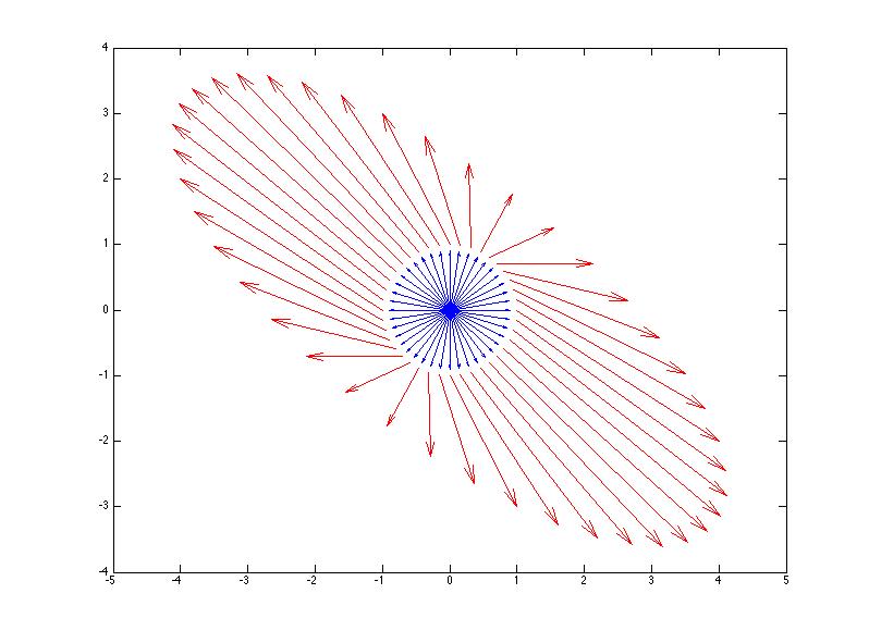
Figure 12.1: Visualizing eigenvectors (in black) using the image (in red) of the unit sphere (in blue) after multiplication by \(\A\).

12.3 Exercises

1. Show that \(\v\) is an eigenvector of \(\A\) and find the corresponding eigenvalue:
   1. $= & 2 \2 & 1 \-3 $
   2. $= & 1 \6 & 0 \-2 $
   3. $= & -2 \5 & -7 \2 $
2. Show that \(\lambda\) is an eigenvalue of \(\A\) and list two eigenvectors corresponding to this eigenvalue:
   1. \(\A=\pm 0& 4\\-1&5\mp \quad \lambda = 4\)
   2. \(\A=\pm 0& 4\\-1&5\mp \quad \lambda = 1\)
3. Based on the eigenvectors you found in exercises 2, can the matrix \(\A\) be diagonalized? Why or why not? If diagonalization is possible, explain how it would be done.
4. Can a rectangular matrix have eigenvalues/eigenvectors?