Chapter 17 Applications of SVD
17.1 Latent Semantic Indexing
17.2 Image Compression
17.2.1 Image data in R
Let’s take an image of a leader that we all know and respect:

Figure 17.1: Michael Rappa, PhD, Founding Director of the Institute for Advanced Analytics and Distinguished Professor at NC State
This image can be downloaded from the IAA website, after clicking on the link on the left hand side “Michael Rappa / Founding Director.”
Let’s read this image into R. You’ll need to install the pixmap package:
#install.packages("pixmap")
library(pixmap)
Download the image to your computer and then set your working directory in R as the same place you have saved the image:
setwd("/Users/shaina/Desktop/lin-alg")The first thing we will do is examine the image as an [R,G,B] (extension .ppm) and as a grayscale (extension .pgm). Let’s start with the [R,G,B] image and see what the data looks like in R:
rappa = read.pnm("LAdata/rappa.ppm")## Warning in rep(cellres, length = 2): 'x' is NULL so the result will be NULL#Show the type of the information contained in our data:
str(rappa)## Formal class 'pixmapRGB' [package "pixmap"] with 8 slots
## ..@ red : num [1:160, 1:250] 1 1 1 1 1 1 1 1 1 1 ...
## ..@ green : num [1:160, 1:250] 1 1 1 1 1 1 1 1 1 1 ...
## ..@ blue : num [1:160, 1:250] 1 1 1 1 1 1 1 1 1 1 ...
## ..@ channels: chr [1:3] "red" "green" "blue"
## ..@ size : int [1:2] 160 250
## ..@ cellres : num [1:2] 1 1
## ..@ bbox : num [1:4] 0 0 250 160
## ..@ bbcent : logi FALSEYou can see we have 3 matrices - one for each of the colors: red, green, and blue. Rather than a traditional data frame, when working with an image, we have to refer to the elements in this data set with @ rather than with $.
rappa@size## [1] 160 250We can then display a heat map showing the intensity of each individual color in each pixel:
rappa.red=rappa@red
rappa.green=rappa@green
rappa.blue=rappa@blue
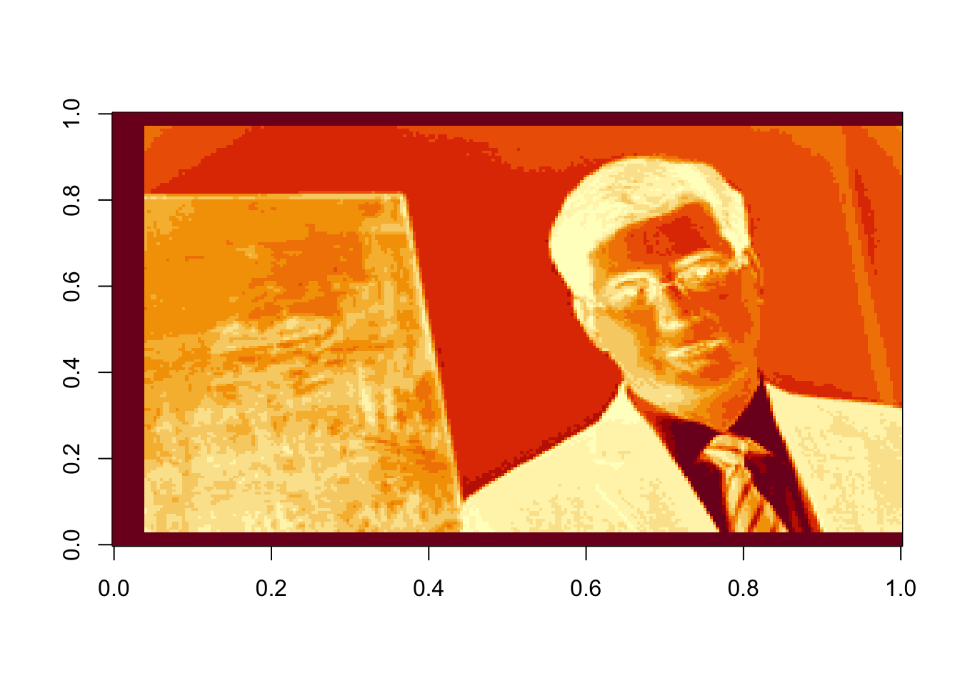
image(rappa.green)
Figure 17.2: Intensity of green in each pixel of the original image
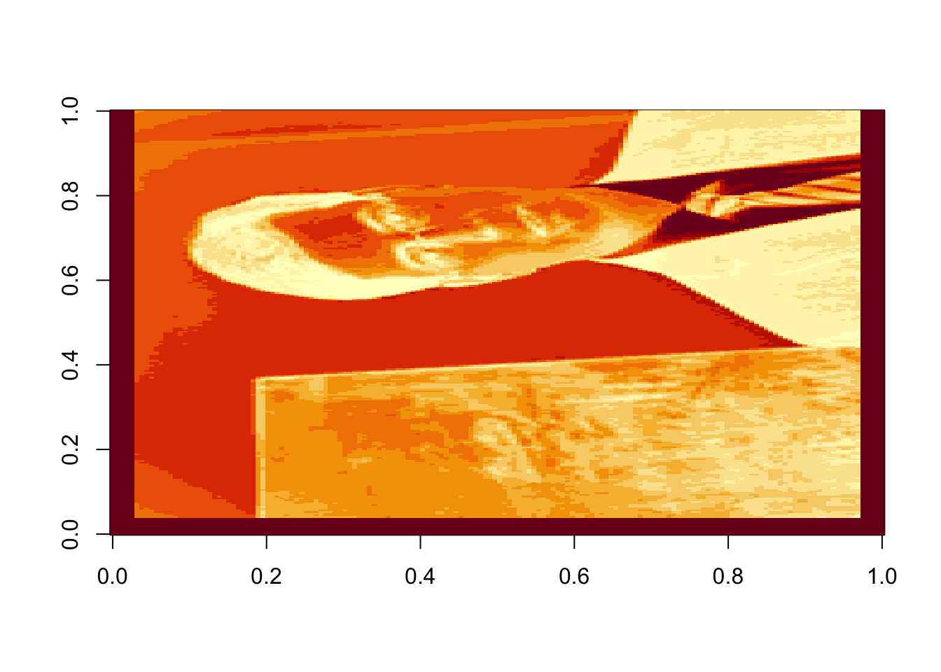
Oops! Dr. Rappa is sideways. To rotate the graphic, we actually have to rotate our coordinate system. There is an easy way to do this (with a little bit of matrix experience), we simply transpose the matrix and then reorder the columns so the last one is first: (note that nrow(rappa.green) gives the number of columns in the transposed matrix)
rappa.green=t(rappa.green)[,nrow(rappa.green):1]
image(rappa.green)
Rather than compressing the colors individually, let’s work with the grayscale image:
greyrappa = read.pnm("LAdata/rappa.pgm")## Warning in rep(cellres, length = 2): 'x' is NULL so the result will be NULLstr(greyrappa)## Formal class 'pixmapGrey' [package "pixmap"] with 6 slots
## ..@ grey : num [1:160, 1:250] 1 1 1 1 1 1 1 1 1 1 ...
## ..@ channels: chr "grey"
## ..@ size : int [1:2] 160 250
## ..@ cellres : num [1:2] 1 1
## ..@ bbox : num [1:4] 0 0 250 160
## ..@ bbcent : logi FALSErappa.grey=greyrappa@grey
#again, rotate 90 degrees
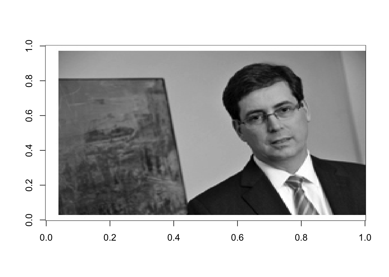
rappa.grey=t(rappa.grey)[,nrow(rappa.grey):1]image(rappa.grey, col=grey((0:1000)/1000))
Figure 17.3: Greyscale representation of original image
17.2.2 Computing the SVD of Dr. Rappa
Now, let’s use what we know about the SVD to compress this image. First, let’s compute the SVD and save the individual components. Remember that the rows of \(\mathbf{v}^T\) are the right singular vectors. R outputs the matrix \(\mathbf{v}\) which has the singular vectors in columns.
rappasvd=svd(rappa.grey)
U=rappasvd$u
d=rappasvd$d
Vt=t(rappasvd$v)
Now let’s compute some approximations of rank 3, 10 and 50:
rappaR3=U[ ,1:3]%*%diag(d[1:3])%*%Vt[1:3, ]
image(rappaR3, col=grey((0:1000)/1000))
Figure 17.4: Rank 3 approximation of the image data
rappaR10=U[ ,1:10]%*%diag(d[1:10])%*%Vt[1:10, ]
image(rappaR10, col=grey((0:1000)/1000))
Figure 17.5: Rank 10 approximation of the image data
rappaR25=U[ ,1:25]%*%diag(d[1:25])%*%Vt[1:25, ]
image(rappaR25, col=grey((0:1000)/1000))
Figure 17.6: Rank 50 approximation of the image data
How many singular vectors does it take to recognize Dr. Rappa? Certainly 25 is sufficient. Can you recognize him with even fewer? You can play around with this and see how the image changes.
17.2.3 The Noise
One of the main benefits of the SVD is that the signal-to-noise ratio of each component decreases as we move towards the right end of the SVD sum. If \(\mathbf{x}\) is our data matrix (in this example, it is a matrix of pixel data to create an image) then,
\[\begin{equation} \mathbf{X}= \sigma_1\mathbf{u}_1\mathbf{v}_1^T + \sigma_2\mathbf{u}_2\mathbf{v}_2^T + \sigma_3\mathbf{u}_3\mathbf{v}_3^T + \dots + \sigma_r\mathbf{u}_r\mathbf{v}_r^T \tag{16.2} \end{equation}\]
where \(r\) is the rank of the matrix. Our image matrix is full rank, \(r=160\). This is the number of nonzero singular values, \(\sigma_i\). But, upon examinination, we see many of the singular values are nearly 0. Let’s examine the last 20 singular values:
d[140:160]## [1] 0.035731961 0.033644986 0.033030189 0.028704912 0.027428124 0.025370919
## [7] 0.024289497 0.022991926 0.020876657 0.020060538 0.018651373 0.018011032
## [13] 0.016299834 0.015668836 0.013928107 0.013046327 0.011403096 0.010763141
## [19] 0.009210187 0.008421977 0.004167310We can think of these values as the amount of ``information’’ directed along those last 20 singular components. If we assume the noise in the image or data is uniformly distributed along each orthogonal component \(\mathbf{u}_i\mathbf{v}_i^T\), then there is just as much noise in the component \(\sigma_1\mathbf{u}_1\mathbf{v}_1^T\) as there is in the component \(\sigma_{160}\mathbf{u}_{160}\mathbf{v}_{160}^T\). But, as we’ve just shown, there is far less information in the component \(\sigma_{160}\mathbf{u}_{160}\mathbf{v}_{160}^T\) than there is in the component \(\sigma_1\mathbf{u}_1\mathbf{v}_1^T\). This means that the later components are primarily noise. Let’s see if we can illustrate this using our image. We’ll construct the parts of the image that are represented on the last few singular components
# Using the last 25 components:

rappa_bad25=U[ ,135:160]%*%diag(d[135:160])%*%Vt[135:160, ]
image(rappa_bad25, col=grey((0:1000)/1000))
Figure 17.7: The last 25 components, or the sum of the last 25 terms in equation (16.2)
# Using the last 50 components:

rappa_bad50=U[ ,110:160]%*%diag(d[110:160])%*%Vt[110:160, ]
image(rappa_bad50, col=grey((0:1000)/1000))
Figure 17.8: The last 50 components, or the sum of the last 50 terms in equation (16.2)
# Using the last 100 components: (4 times as many components as it took us to recognize the face on the front end)

rappa_bad100=U[ ,61:160]%*%diag(d[61:160])%*%Vt[61:160, ]
image(rappa_bad100, col=grey((0:1000)/1000))
Figure 17.9: The last 100 components, or the sum of the last 100 terms in equation (16.2)
Mostly noise. In the last of these images, we see the outline of Dr. Rappa. One of the first things to go when images are compressed are the crisp outlines of objects. This is something you may have witnessed in your own experience, particularly when changing the format of a picture to one that compresses the size.